We downloaded a set of chessboard images from Stanford Light Field Archive. First, we averaged all the images without shifting. Since objects far away from the camera do not vary much in their positions when we shift the camera as nearby objects do, this will create an image that is focused on objects far away but blurry on objects close to the camera. The result is shown as follows.
After that, we extracted the camera positions from the image names, and picked the center image to be the one with index (8, 8). We then calculated the shift distance in both x and y direction from each image to this center image, multiplied the distances by alpha (a number between 0 and 1), shifted each image by those distances, and took the average. Depending on our alpha value, the averaged image will focus on different parts of the chessboard. Namely, larger alpha correspond to closer focuses and vice versa.
Here we present our results.
1.2. Aperture Adjustment
This part is similar to the previous part, except now we define a radius which is effectively our aperture, and we only shift and average images whose camera location is within radius from the center image’s camera location. This implies that a larger radius will produce a blurrier image, which is essentially the same as having a larger aperture.
Below are our results.
R = 0R = 1
R = 2R = 3
R = 4R = 5
R = 6R = 7
R = 8R = 9
R = 10R = 20
1.3. Summary
Overall, light field cameras are really cool, and we are amazed at how we can capture multiple pictures over a plane orthogonal to the optical axis to produce pictures with different depths of view.
2. HDR from multiple LDR images
This project aims to create HDR images using multiple LDR images captured under different exposure. As cameras have a limited dynamic range, in theory multiple exposures can give us a higher dynamic range than one single image could achieve.
2.1 Recovering radiance map from LDR images
The first step is to recreate the relative radiance map from the LDR images. We used the process outlined in the 1997 paper. Each pixel on a sensor or a film can be modeled as a pixel response function where it produces a certain response based on a given input radiance. Any pixel value on a image can be modeled by such function g(lEδt), where the δt is the exposure. If we take the log of this function this can be transformed to log(lE)+log(δt). This way we can use different exposures of images (with different δt) to fit a function for g. Usually we can’t solve for this function, but in this case as the pixel values are limited and discreet, we can solve it as a system of linear equations.
Here’s the plot of recovered pixel response function of R, G, and B. The empty circles in the background are the supporting data points and the solid curve is the fitted response function.
Note that for this image set, as it is scanned from films, it does not have perfect black level. In fact the black level is a non zero value, so we observe a deviation from the response curve to the actual image. For another set of images taken by a modern DLSR, this curve is much cleaner.
Here’s the recovered radiance image:
Here’s the original image set that produces this radiance:
2.2 Tone-mapping
After we got the radiance map, we can not just directly display such radiance as our display also have a limited dynamic range. We need to tone-map this image into our display space.
For sanity check, we first directly compute the log of the image and then rescaled the image to an output space of 0 to 1. This gives us:
Then we tried a famous and simple global tonemapper: Reinhard tonemapping:
The image produced is very nice, although the highlights are a bit blown out and not showing the accurate color. (However I personally favor this as this is more realistic to human vision)
Then we moved on to implementing global tonemapping.
We first need to convert the radiance back to log space, and then compute two seperate maps: one for the details, one for the lower frequency information. Instead of directly using gaussian blur, the algorithm used in Durand (2002) uses bilateral filtering to eliminate possible haloing.
This produces two maps:
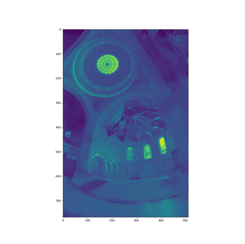
The low frequency:
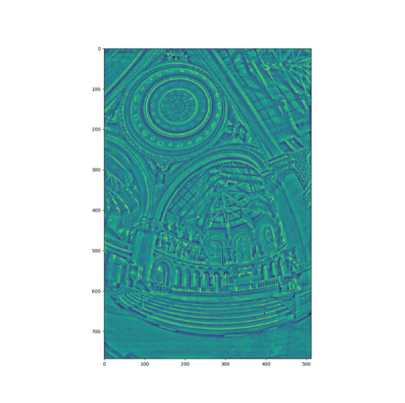
The details map (high frequency):
The approach of this local tone mapping method is try to scale the low frequency into a limited dynamic range, while the higher frequency retains their dynamic range. This produces results with much larger dynamic range but it utilizes human’s color perception (which is local) to recreate the effect for a larger dynamic range.
All the outputs are then converted back to linear space. (This step is also included in the previous two global tone mapping algorithm.) As the sRGB color format is in a gamma space, we need to use the gamma curve (power of 2.2) to adjust our linear space image into the display space so that the linear response are perceptually linear. All these combined produced the result:
2.3 Testing this on our own image
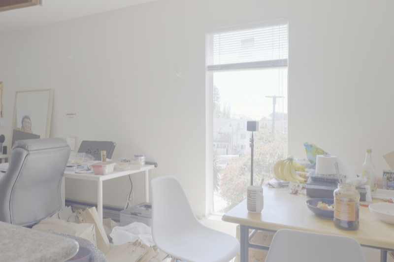
We captured an indoor scene during afternoon where very bright sunlight poured in and there’s a huge dynamic range difference in the image.
Here’s the set of original images:
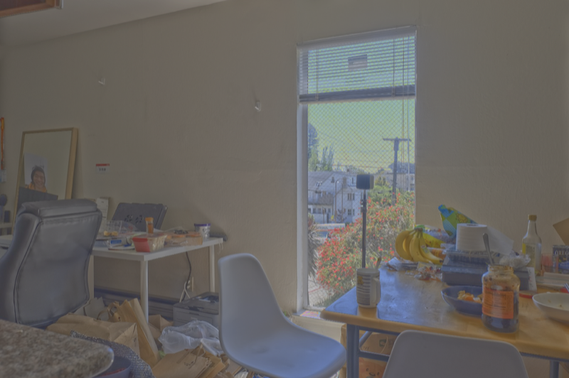
And here are the results:
Log tone mapping (global)
Reinhard mapping (global)
Durand 2002 (local)
It seems that there’s some false color in the extremely bright area, this is likely due to we don’t have enough dynamic range in the original images and we can’t recover the radiance from the highlights. The original images are taken in one stop gap between each other (two times amount of light), and it results in 7 stops of dynamic range. Each image itself contains roughly 7 stops of dynamic range, resulting in an image with 14 stops of dynamic range. It seems like 14 stops is still not enough for this scene. Compressing such large dynamic range do causes the image to lose the sense of shadow and light. Maybe it’s caused by too small of a bilateral filter.
3. A Neural Algorithm of Artistic Style
For this project, we re-implemented the neural style transfer with PyTorch as described in this paper. We used the pretrained VGG-19 network.
First, we preprocessed the image by normalizing by the mean and standard deviation of the VGG training dataset. We resized our style images to be the same sizes as our content images. We also made both the content and style images to be of batch size 1 in order to match the input shape of VGG-19.
Then, we defined our content and style loss according to the paper, and to make the images look nicer, we also added the total variation loss to the total loss. At first, we used the second conv2d layer of after the third max pool layer for content loss, and all five conv2d layers after max pooling layers for our style loss (each with weight 1/5). We defined the ratio of the content loss weight to the style loss weight to be 1e-3 as specified in the paper. However, this produced undesirable results.
This is a image showing this, the style picture is starry night and the content picture is tubingen:
To improve our results, we decided to follow PyTorch’s tutorial and use the 4th conv2d layer for content loss, and the first 5 conv2d layers for style loss.
Here’s an image produced using the style of muse and a content of a picture of Cory hall:
We observed that the colors of the image matched the colors of the style image, but as training progresses basically only the color is reproduced and the picture gets less colorful as the training progresses on. We suspected that this is a problem with the weights on different loss, and we printed the three different loss functions to check. We found that the style loss is no longer being optimized and it’s basically the same throughout the training. We decided to adjust the weights.
In the end, after a lot of parameter tuning, we decided on a content weight of 10−6, a style weight of 1500 for each layer, and a total variance weight of 10−5. This finally produces the result we want.
During the training process, we observed that it takes a long time for Adam to optimize the image, and we need to tune the learning rate, decreasing it after a certain iterations. We decided to use L-BFGS optimizer instead of Adam, as L-BFGS uses a pseudo-newton method that approximates a hessian matrix. This leads to very fast training, but it comes with a cost of extremely high memory usage. This is fine for our case as the neural style transfer only ever optimizes one image.
CS 194 Final Project Report
Group Members
Table of Contents
1. Light Field Camera
1.1. Depth Refocusing
We downloaded a set of chessboard images from Stanford Light Field Archive. First, we averaged all the images without shifting. Since objects far away from the camera do not vary much in their positions when we shift the camera as nearby objects do, this will create an image that is focused on objects far away but blurry on objects close to the camera. The result is shown as follows.
After that, we extracted the camera positions from the image names, and picked the center image to be the one with index (8, 8). We then calculated the shift distance in both x and y direction from each image to this center image, multiplied the distances by
alpha(a number between 0 and 1), shifted each image by those distances, and took the average. Depending on ouralphavalue, the averaged image will focus on different parts of the chessboard. Namely, largeralphacorrespond to closer focuses and vice versa.Here we present our results.
1.2. Aperture Adjustment
This part is similar to the previous part, except now we define a
radiuswhich is effectively our aperture, and we only shift and average images whose camera location is withinradiusfrom the center image’s camera location. This implies that a largerradiuswill produce a blurrier image, which is essentially the same as having a larger aperture.Below are our results.
1.3. Summary
Overall, light field cameras are really cool, and we are amazed at how we can capture multiple pictures over a plane orthogonal to the optical axis to produce pictures with different depths of view.
2. HDR from multiple LDR images
This project aims to create HDR images using multiple LDR images captured under different exposure. As cameras have a limited dynamic range, in theory multiple exposures can give us a higher dynamic range than one single image could achieve.
2.1 Recovering radiance map from LDR images
The first step is to recreate the relative radiance map from the LDR images. We used the process outlined in the 1997 paper. Each pixel on a sensor or a film can be modeled as a pixel response function where it produces a certain response based on a given input radiance. Any pixel value on a image can be modeled by such function g(lEδt), where the δt is the exposure. If we take the log of this function this can be transformed to log(lE)+log(δt). This way we can use different exposures of images (with different δt) to fit a function for g. Usually we can’t solve for this function, but in this case as the pixel values are limited and discreet, we can solve it as a system of linear equations.
Here’s the plot of recovered pixel response function of R, G, and B. The empty circles in the background are the supporting data points and the solid curve is the fitted response function.
Note that for this image set, as it is scanned from films, it does not have perfect black level. In fact the black level is a non zero value, so we observe a deviation from the response curve to the actual image. For another set of images taken by a modern DLSR, this curve is much cleaner.
Here’s the recovered radiance image:
Here’s the original image set that produces this radiance:
2.2 Tone-mapping
After we got the radiance map, we can not just directly display such radiance as our display also have a limited dynamic range. We need to tone-map this image into our display space.
For sanity check, we first directly compute the log of the image and then rescaled the image to an output space of 0 to 1. This gives us:
Then we tried a famous and simple global tonemapper: Reinhard tonemapping:
The image produced is very nice, although the highlights are a bit blown out and not showing the accurate color. (However I personally favor this as this is more realistic to human vision)
Then we moved on to implementing global tonemapping.
We first need to convert the radiance back to log space, and then compute two seperate maps: one for the details, one for the lower frequency information. Instead of directly using gaussian blur, the algorithm used in Durand (2002) uses bilateral filtering to eliminate possible haloing.
This produces two maps:
The low frequency:
The details map (high frequency):
The approach of this local tone mapping method is try to scale the low frequency into a limited dynamic range, while the higher frequency retains their dynamic range. This produces results with much larger dynamic range but it utilizes human’s color perception (which is local) to recreate the effect for a larger dynamic range.
All the outputs are then converted back to linear space. (This step is also included in the previous two global tone mapping algorithm.) As the sRGB color format is in a gamma space, we need to use the gamma curve (power of 2.2) to adjust our linear space image into the display space so that the linear response are perceptually linear. All these combined produced the result:
2.3 Testing this on our own image
We captured an indoor scene during afternoon where very bright sunlight poured in and there’s a huge dynamic range difference in the image.
Here’s the set of original images:
And here are the results:
Log tone mapping (global)
Reinhard mapping (global)

Durand 2002 (local)
It seems that there’s some false color in the extremely bright area, this is likely due to we don’t have enough dynamic range in the original images and we can’t recover the radiance from the highlights. The original images are taken in one stop gap between each other (two times amount of light), and it results in 7 stops of dynamic range. Each image itself contains roughly 7 stops of dynamic range, resulting in an image with 14 stops of dynamic range. It seems like 14 stops is still not enough for this scene. Compressing such large dynamic range do causes the image to lose the sense of shadow and light. Maybe it’s caused by too small of a bilateral filter.
3. A Neural Algorithm of Artistic Style
For this project, we re-implemented the neural style transfer with PyTorch as described in this paper. We used the pretrained VGG-19 network.
First, we preprocessed the image by normalizing by the mean and standard deviation of the VGG training dataset. We resized our style images to be the same sizes as our content images. We also made both the content and style images to be of batch size 1 in order to match the input shape of VGG-19.
Then, we defined our content and style loss according to the paper, and to make the images look nicer, we also added the total variation loss to the total loss. At first, we used the second conv2d layer of after the third max pool layer for content loss, and all five conv2d layers after max pooling layers for our style loss (each with weight 1/5). We defined the ratio of the content loss weight to the style loss weight to be 1e-3 as specified in the paper. However, this produced undesirable results.
This is a image showing this, the style picture is starry night and the content picture is tubingen:
To improve our results, we decided to follow PyTorch’s tutorial and use the 4th conv2d layer for content loss, and the first 5 conv2d layers for style loss.
Here’s an image produced using the style of muse and a content of a picture of Cory hall:
We observed that the colors of the image matched the colors of the style image, but as training progresses basically only the color is reproduced and the picture gets less colorful as the training progresses on. We suspected that this is a problem with the weights on different loss, and we printed the three different loss functions to check. We found that the style loss is no longer being optimized and it’s basically the same throughout the training. We decided to adjust the weights.
In the end, after a lot of parameter tuning, we decided on a content weight of 10−6, a style weight of 1500 for each layer, and a total variance weight of 10−5. This finally produces the result we want.
During the training process, we observed that it takes a long time for Adam to optimize the image, and we need to tune the learning rate, decreasing it after a certain iterations. We decided to use L-BFGS optimizer instead of Adam, as L-BFGS uses a pseudo-newton method that approximates a hessian matrix. This leads to very fast training, but it comes with a cost of extremely high memory usage. This is fine for our case as the neural style transfer only ever optimizes one image.
Here are some results:
Image of cory hall, with style of muse:
Image of tubingen, with style of the scream:
Image of tubingen, with style of starry night: