CS194 Final Projects:

Seam Carving & Lightfield Camera

Ahmed Malik || Spring 2020

Project 1: Seam Carving

Overview

In this project we follow the algorithm proposed by Avidan and Shamir in Seam Carving for Content-Aware Image Resizing in order to shrink (and enlarge for Bells & Whistles) images. A seam is defined as a path of adjacently connected pixels along solely either the vertical or horizontal axes of an image. Unlike methods that simply rescale an image considering just geometric constraints, this algorithm shrinks (or enlarges) an image by considering the content of the image: it removes (or inserts) pixels based on their energy. Therefore, a seam is determined by computing paths of low energy along the axes of an image.

Computing the Energy of an Image

We can imagine that the energy of an image would indicate which subjects in the scene hold the most weight. For this reason, Avidan and Shamir intuit that an effective energy function would allow for the removal of unnoticeable pixels that blend with their surroundings. Therefore, following their method, we define the energy function to be the gradient of the image in the x and y directions:

e (I) = | \frac{\partial}{∂x} I | + | \frac{\partial}{∂y} I |

We implement this similar to Project 2, by performing a convolution with the image and Dx and Dy operators respectively:

D_{x} = [\begin{matrix} 1 & -1 \end{matrix}]

D_{y} = [\begin{matrix} 1 \\ -1 \end{matrix}]

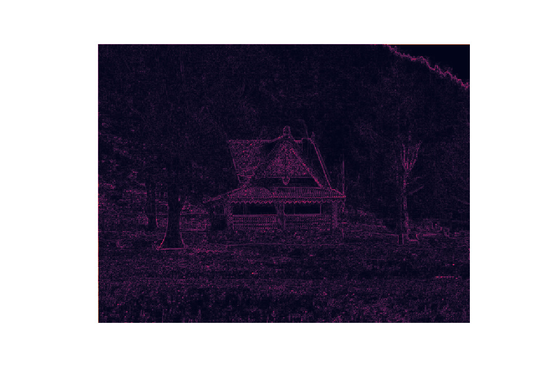
If we look at the gradient, we're effectively left with the edges of the subject matter in the original image:

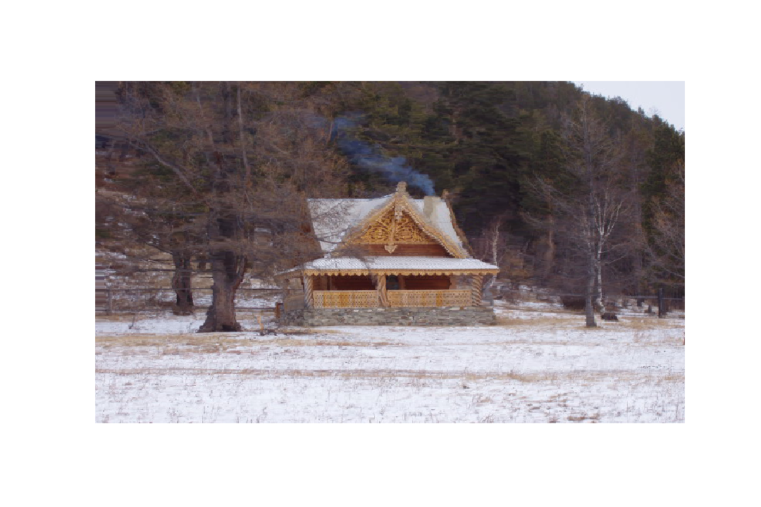
Looking at this, we expect the house to remain relatively unaffected during seam operations when compared to the trees.

Finding the Optimal Seam

Avidan and Shamir define the optimal seam $s^{*}$ as:

s^{*} = \sum_{i = 1}^{n} e (I (s_{i}))

The optimal seam can be found using dynamic programming and the method is broken down into two steps. First, we traverse the image from the second row to the last row and compute the cumulative minimum energy matrix $M$ for all possible connected seams for each pixel $(i, j)$ . Consequently, the minimum value (minimum column) in the last row of $M$ indicates the end of the minimal connected vertical seam. Thus, second, we can backtrack from this point to find the the entire minimal connected seam. We compute $M$ as follows, where $e$ is the matrix of the energy of each pixel in $I$ , computed using the energy function (gradient of image):

M (i, j) = e (i, j) + \min (M (i - 1, j - 1), M (i - 1, j), M (i - 1, j + 1)

Note that the first row of the $M$ matrix is set as $M (0, 0) = e (0, 0)$ .

To remove the seam, we create a 2D mask filled with 1's except for the $(i, j)$ points corresponding to the minimal seam, which are set to 0. Then, we flatten both the mask and image to 1D, apply the mask to the image, and reshape the image back to 2D.

The process for finding the optimal horizontal seam is exactly the same as finding the vertical seam, but the input image to the algorithm is the transpose of the original image. After the seams are removed from the transposed image, the final image is transposed again to its correct orientation.

Results

Here are examples of where the algorithm performed well: 150 vertical seams removed

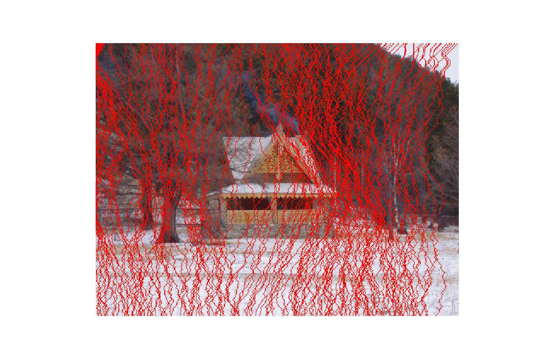
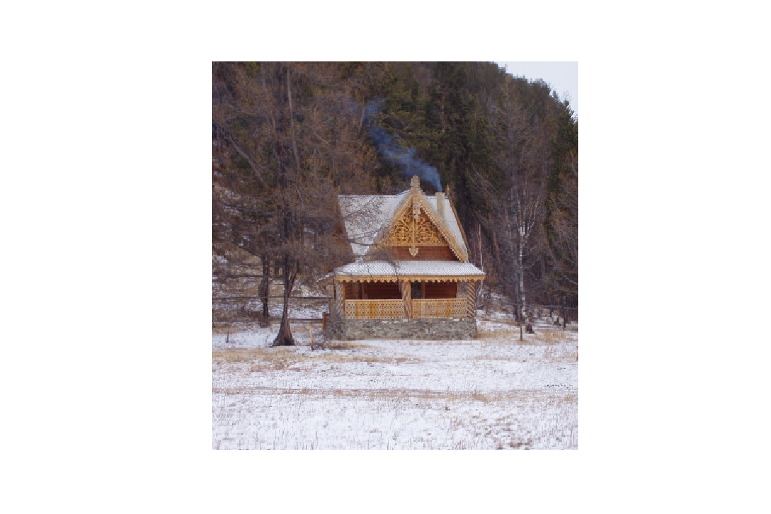
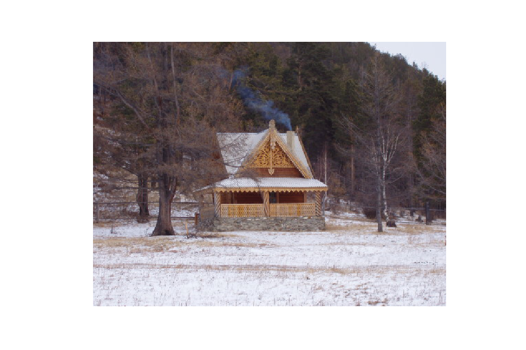
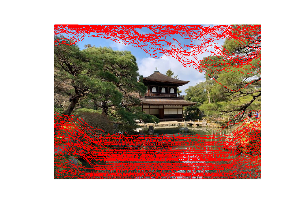
The algorithm performs well shrinking this image of a house in a forest horizontally. Though the seams (marked in red) are spread across the whole image, they are more sparse on the features of the house as compared to the trees. The resulting image doesn't shrink the house too much, but we notice significant reduction in the width of the tree to the left of the house. The large, emtpy spaces of forest are significantly reduced to the right of the house as well.

250 vertical seams removed

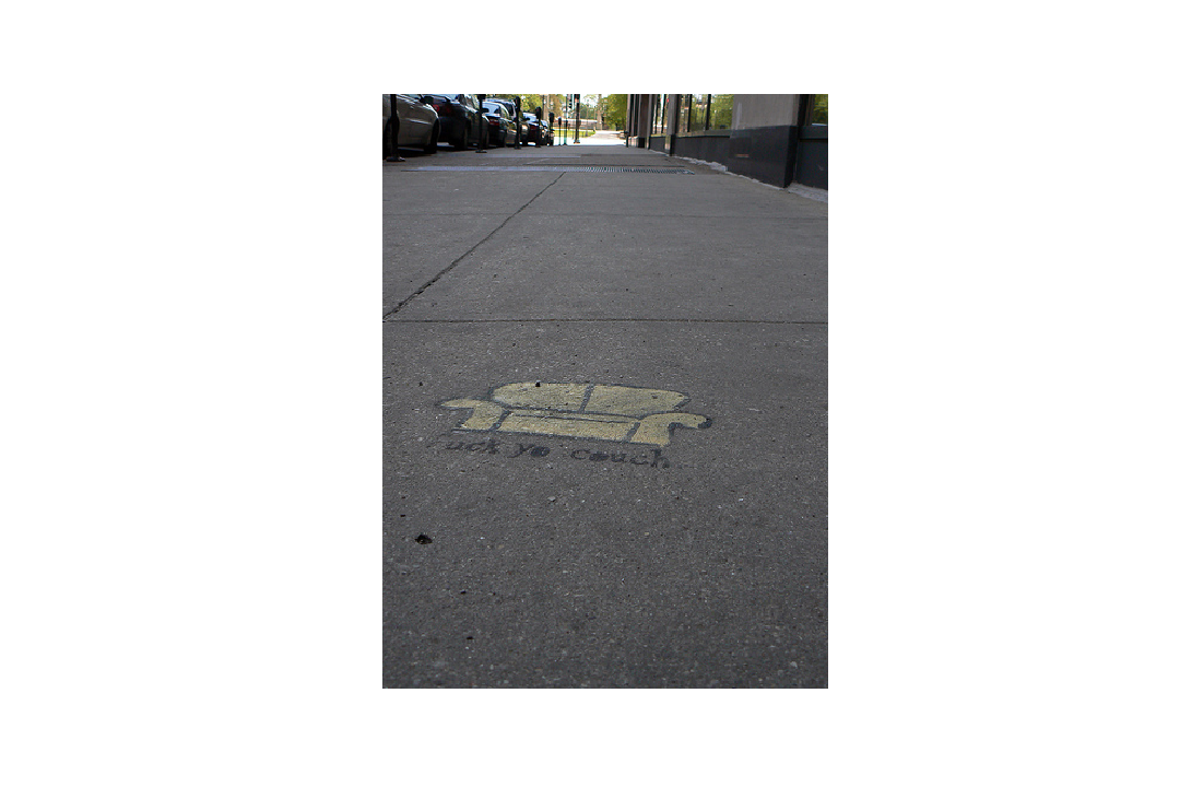
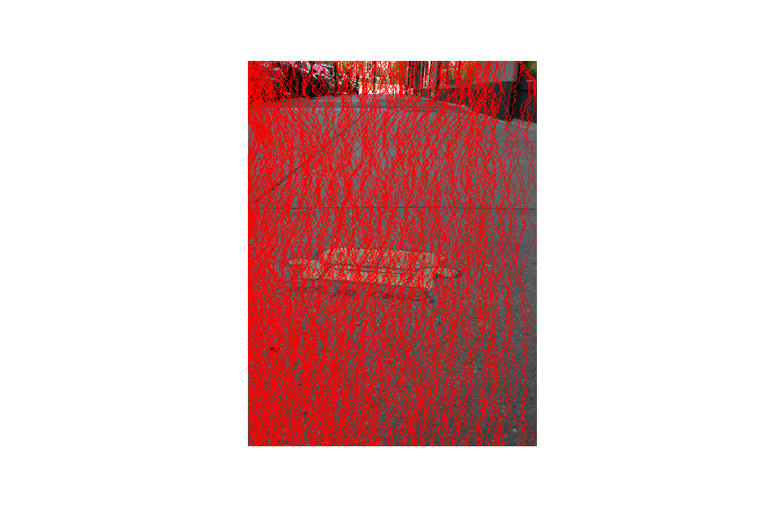
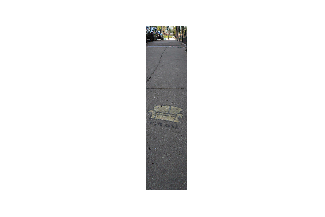
Considering how significant the removal of 250 vertical seams is for this image, the algorithm performs exceptionally well, maintaining the salient features of couch graffiti (primary subject matter). The background is also kept reasonably intact without much noticeable distortion.

250 horizontal seams removed

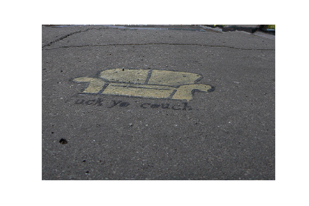
Removing 250 horizontal seams really helps to focus the image onto the couch graffiti (primary subject matter) and effectively crops out the upper portion of the image. It is curious that the pavement right above the couch is considered higher energy than the horizontal paths along the couch graffiti.

250 horizontal seams removed

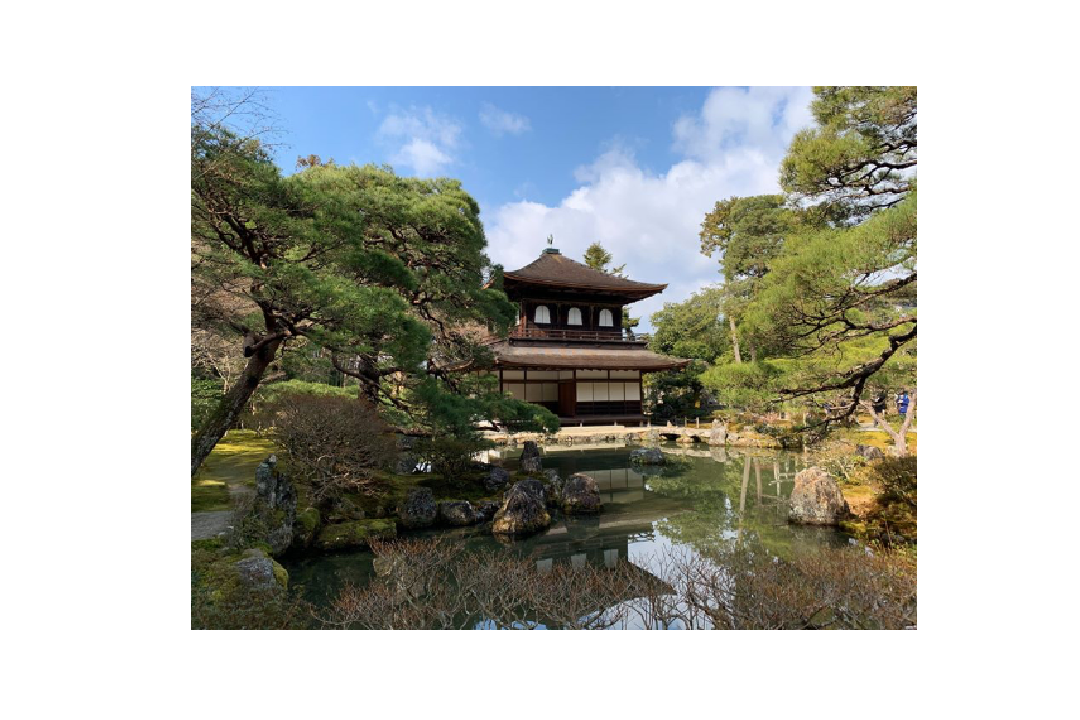
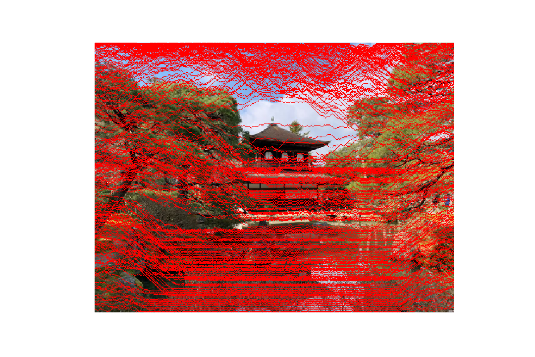
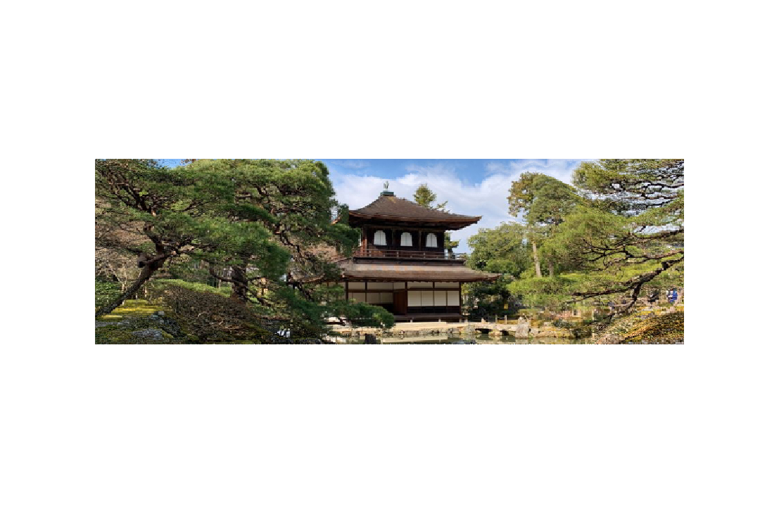
For the pagoda image, we remove a significant number of horizontal seams to shrink the image vertically, and we notice that the pagoda itself (primary subject matter) is mostly unaffected. The foreground of the pond is effectively cropped out.

250 vertical seams removed

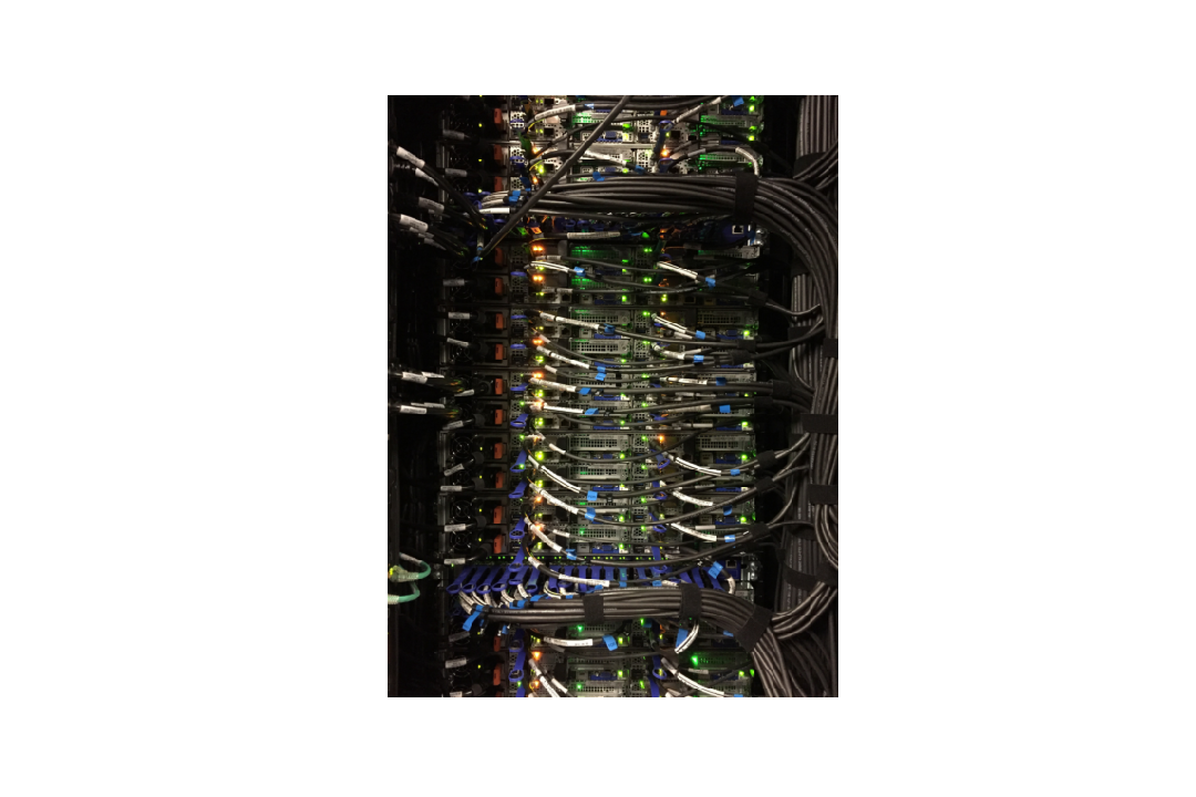
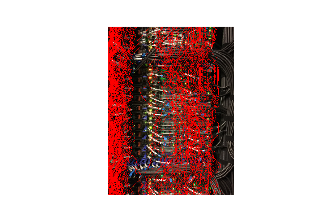
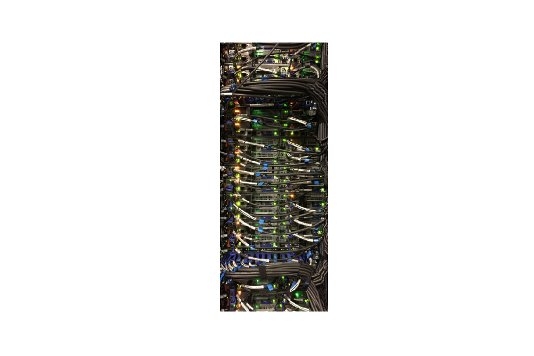
For the server image, the algorithm does a good job shrinking horizontally. It effectively crops out the dark, unnecessary portion towards the left of the image, and shrinks the right portion of the image with minimal distortion on the rightmost wires.

270 horizontal seams removed

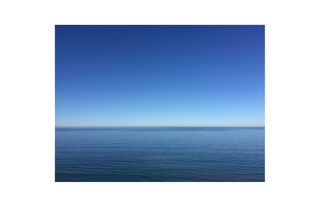
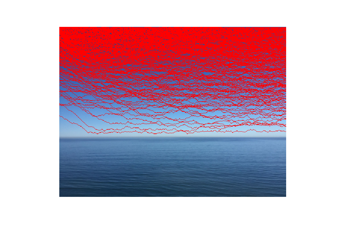
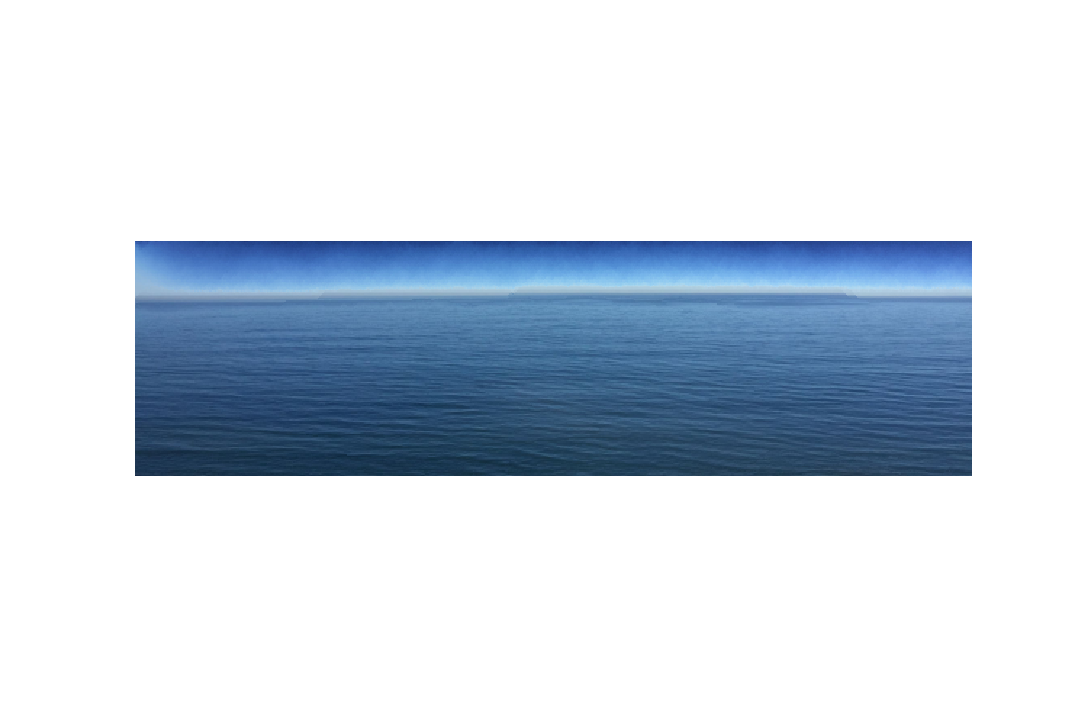
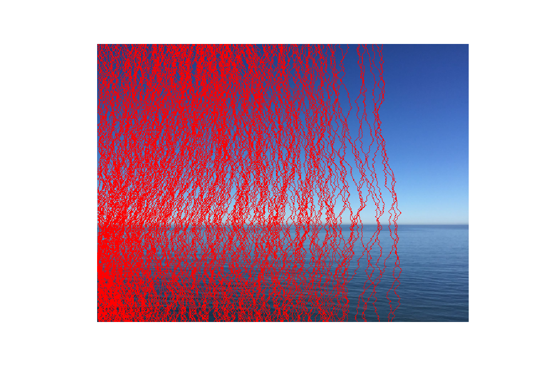
We expect the algorithm to perform very well here considering the subject matter is very simple. The energy function computes that the ocean has much higher energy than the sky, so the sky is almost entirely cropped out, leaving mostly just the horizon. Almost no distortion is discernable due to how similar the sky pixels all are.

Bells & Whistles: Enlarging Images Using Seam Insertion

Above, we've shown that using seam carving we can shrink an image either vertically or horizontally. Here, we extrapolate this to enable enlarging images.

In order to retain the original features of the primary subject matters, we wish to add the $k$ seams of lowest energy. By doing this, we only add pixels that were already relatively unnoticeable due to blending in with their surroundings. Relative to pixels of higher energy, adding more lower energy pixels will negligibly affect the result of the enlarged image.

However, we must be careful about inserting and computing seams of low energy. As Figure 8b of Avidan and Shamir shows, adding a seam and then recomputing the lowest energy seam to add will likely result in the same seam being added over and over again. To get around this, we first go through the seam removal process as normal, but keep track of all $k$ seams being removed. Once these $k$ seams are determined, all that's left to do is add these seams to the original image. To make the result smoother, we average the pixels in the column direction one before and one after for the $(i, j)$ pixels of the seam being added:

I^{'} (i, s_{k}^{*} [i] + 1) = avg (I (i, s_{k}^{*} [i]), I (i, s_{k}^{*} [i] + 1), I (i, s_{k}^{*} [i] + 2))

s_{k}^{*} [i] = 0

I^{'} (i, s_{k}^{*} [i]) = avg (I (i, s_{k}^{*} [i] - 1), I (i, s_{k}^{*} [i]), I (i, s_{k}^{*} [i] + 1))

otherwise where

s_{k}^{*} [i]

is the

k^{th}

seam of lowest energy for all rows

i

, and

I^{'}

is the new, enlarged image.

Image enlargement performed well in these results:

125 horizontal seams added

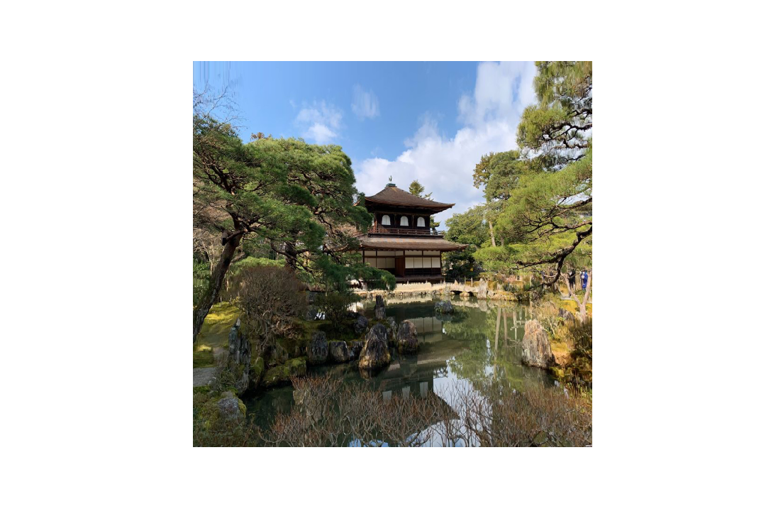
The image of the pagoda is vertically enlarged by 125 seams. The pagoda itself is completely untouched, but portions of the lower energy sky and pond are readded to the image to make it appear larger without (much) distortion. The branches at the top left are very slightly strethced.

200 horizontal seams added

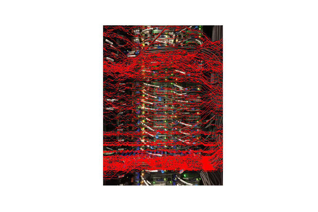
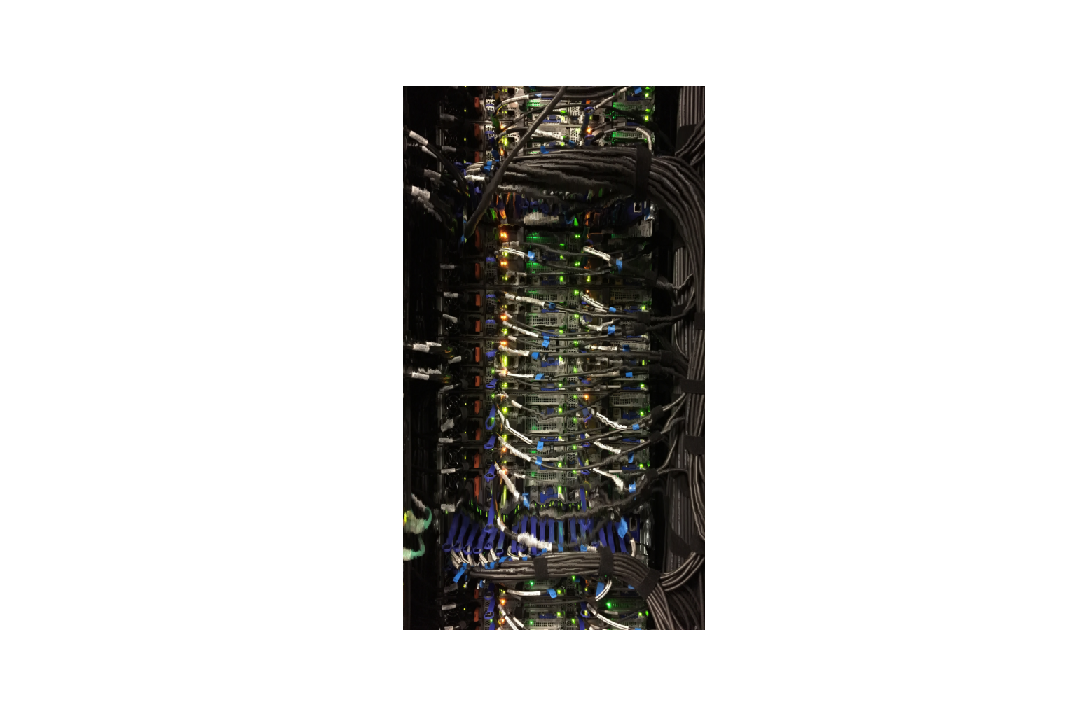
The image of the server is vertically enlarged by 200 seams. Without zooming in, the image looks normal, and achieves the effect of stretching vertically. The majority of the image is stretched in areas of that aren't near the center, and the center is stretched very slightly, but uniformly. As such, the image mostly retains its "signal-to_noise-ratio", so to speak. However, zooming in does show the image exhibits mild effects of distortion, especially along the bottom and top wires, but nothing significant.

150 vertical seams added

Here, we stretch the image of the house in the forest horizontally by adding vertical seams. As shown in red, the seams are mostly uniformly spread across the width of the image, so the subject matters of the enlarged image simply looks strecthed (or scaled) in width, but the image doesn't look distorted. Similar to the enlarged server image, the "signal-to-noise" ratio is relatively maintained because the stretch happens uniformly across the width.

270 vertical seams added

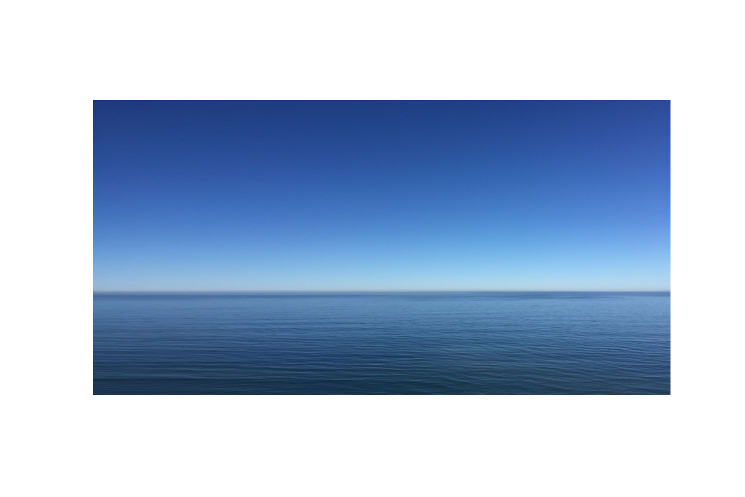
The image of the ocean is stretched horizontally and shows no sings of distortion at all. A significant amount of seams are added from the left side of the image, becoming slightly sparser as the seams move towards the right. Again, this is a fairly uniform stretch, but even without the uniformity we could expect this image would perform well in enlargement (just as it did in shrinkage) because of how simple the scenery is.

Failed Results

The following are examples of images shrunk or enlarged that exhibited significant distortion:

270 vertical seams removed

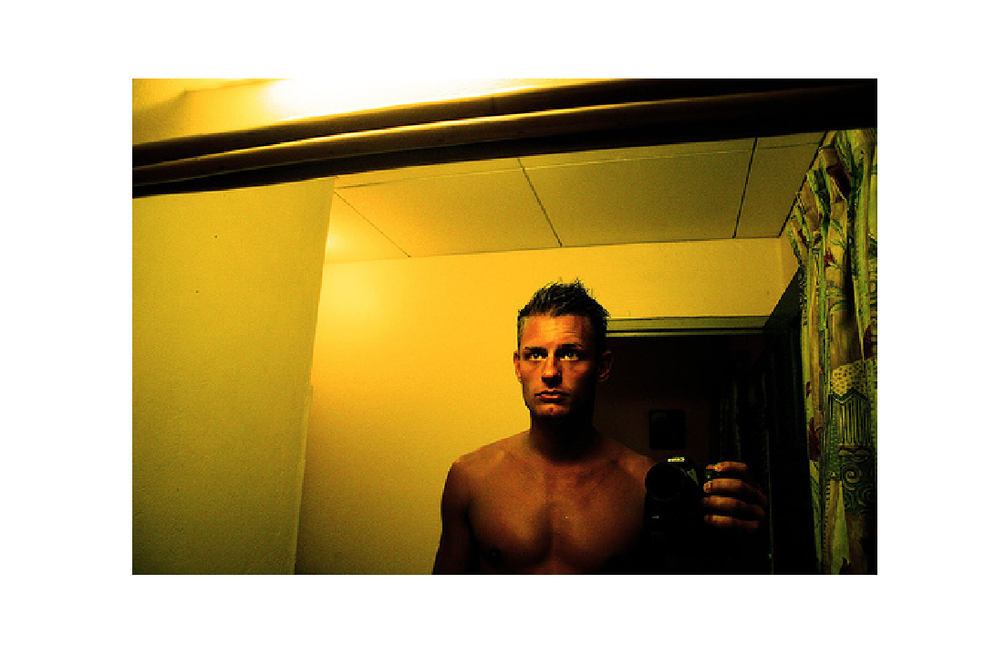
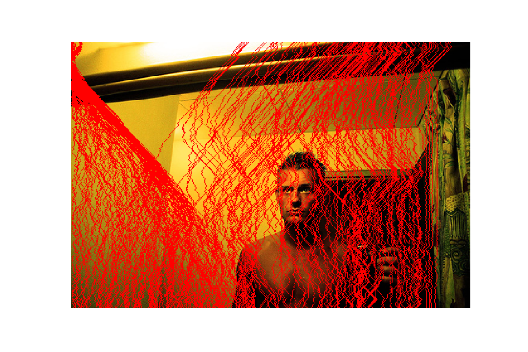
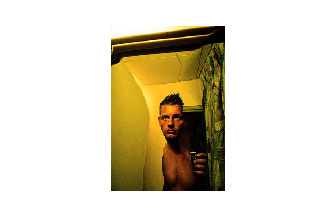
The man in the portrait is a signficant component of the composition of the image, but due to the lighting in the environment, the sides of his body have much lower intensity and so are paths of lower energy. Hence, much of his body is distorted (squished), while the curtains remain almost entirely unaffected.

150 vertical seams removed

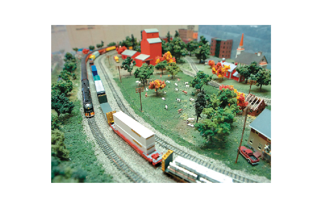
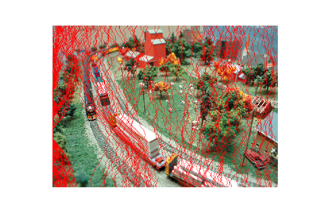
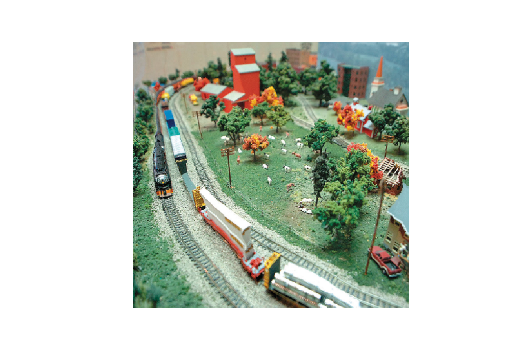
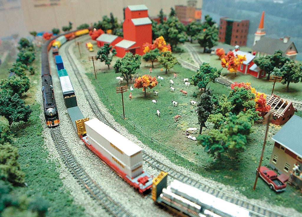
The trains are a key component of the composition of this image and although most seams removed are spread uniformly across the width of the image, the trains are siginficantly affected because they are thin objects. As such, even a small amount of seams affecting a train can have a large effect, especially farther back in the image. This is why we see the white and black trains exhibit significant distortion where they appear squished in width.

Final Thoughts

I found the core idea of this project -- computing a path of low energy pixels (seam) -- to be very cool and important. It introduced me to the idea of resizing an image by being "content-aware", whereas in the past I had simply thought of resizing to be an operation applied equally throughout all pixels. I think it's really cool that with a simple energy function we can find seams in an image and remove these to get rid of sparse areas or the negative space in an image.

Image Attributions

House, couch graffiti, self portrait
Train
Pagoda, Server, Ocean: Personal

Project 2: Lightfield Camera

Overview

Taking inspiration from this paper by Ren Ng et al., in this project, we aim to mimic the effects of a lightfield camera in software. This will allow the user two different controls: depth refocusing and aperture adjustment. In a normal camera, these two properties are set before snapping a picture, and once the image is snapped, there is no way to shift the focus to different areas of the image, or alter the aperture size in post. However, if the user is able to snap pictures of the same subject matter from multiple angles across a grid, the set of images could be averaged together and shifted to simulate focus at different depths and differet aperture size.

We acquire lightfield data from the Stanford Light Field Archive. We use the images taken on a 17x17 grid for this project.

Depth Refocusing

As the camera moves across the 289 points of the 17x17 grid, the position of the objects in the scene closer to the camera vary greater than the objects further from the camera. If we naively average all images in the grid without accounting for the shift in position, the objects further from the camera will remain in focus while the objects in the foreground will blur due to the relative shift. To correct this, before averaging images together, we first shift them to a common reference point, and then overlay them together for averaging. The common reference point we use here is the center of the grid, at a coordinate of $(u_{ref}, v_{ref}) = (8, 8)$ . Therefore, we define the new, shifted grid coordinate $(u^{'}, v^{'})$ of each image to be:

(u^{'}, v^{'}) = ((c * (u - u_{ref}), c * (v - v_{ref}))

where

c

is the scaling constant used to move the depth of the focus. Through testing, we found that scaling factors of 0 to 3 worked well, with 0 used to focus the objects further away (background), and 3 used to focus the objects closer (foreground). The following are two examples of depth refocusing using scaling constants from 0 to 3, spaced evenly by 0.2:

We see in both gifs that the focus moves from the background to the foreground as the scaling factor increases. The effect is more clearly noticeable in the chessboard, which the Stanford Light Field Archive notes is a great example for demonstrating refocusing.

Aperture Adjustment

The size of the aperture controls the amount of light being used to form the image. As the aperture of a camera increases to let in more light, more light rays from multiple angles are able to reach the photo sensor, resulting in a blurrier image. We can simulate this with the lightfield camera by likening each image on the 17x17 grid as an image taken by a pinhole camera from that viewpoint. Building off of this, we can simulate a larger aperture by increasing the number of images averaged together within some max distance $d_{\max}$ from some reference viewpoint $(u_{ref}, v_{ref})$ on the 17x17 grid. Items perpendicular to the plane of the camera will remain in focus because their light rays are all nearly perpendicular to the camera plane to begin with, and so after they pass the "pinhole", they won't veer off much from their original position. Items towards the edges of the camera view will have much more significant deviation when they hit the photo sensor plane.

To achieve this, we select some referene point $(u_{ref}, v_{ref})$ and find the subset of all images within some max distance $d_{\max}$ by computing the distance for each viewpoint along the grid $d_{(u,v)}$ using Euclidean distance:

d_{(u,v)} = \sqrt{(u - u_{ref})^{2} + (v - v_{ref})^{2}}

Then, for each subset of images within some

d_{\max}

, we overlay and average them together. Below are the results of this on two lightfield datasets:

The chess gif is using a reference point on the grid of $(u_{ref}, v_{ref}) = (15, 15)$ and goes through a range of $d_{\max} = [1, 22]$ , while the jelly-beans gif is centered at $(u_{ref}, v_{ref}) = (8, 8)$ and goes through a range of $d_{\max} = [1, 12]$

For fun, here is an animation showing both depth refocusing and aperture at the same time, for the same configuration of the chess lightfield dataset as above:

Summary

This project was extremely cool and really helped me understand the fundamentals behind depth control/focus and aperture control in a camera. In particuar, the idea that a simulated light field can be broken down into a pinhole camera at a single viewpoint is really interesting. I enjoyed how intuitive and simple the idea behind a grid to simulate a light field is, and how powerful it can be to enable altering the focus of an image in post.