sukrit.arora@berkeley.edu, cs194-26-ahb)suraj.rampure@berkeley.edu, cs194-26-adz)We did three projects together:
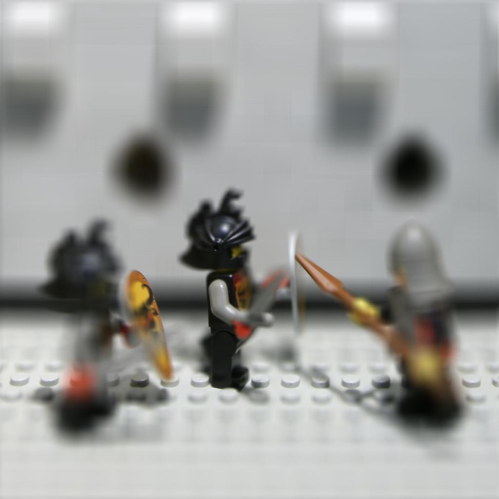
In this project, we used images from the Stanford Light Field Archive to simulate depth refocusing and aperture adjustment.
Each “image” in the above dataset consisted of 289 sub-images, or sub-apertures. These could be arranged in a 17 by 17 grid, with the image at (8, 8) being at the center. Averaging these images in different ways will allow us to re-create the desired results.
To change the depth of focus, one needs to “shift” all images that are off-center by some amount, and then average them all. Specifically, the shifts applied to the image at position in the aforementioned grid are given by
We used np.roll to do our shifting; the cyclic artifacts were small enough to ignore since the shifts were relatively small. After averaging all 289 shifted images, the result is a new image whose depth of focus depends on the constant, . Here are both of them with :
Varying within some range allows us to change the depth of focus and create a gif.
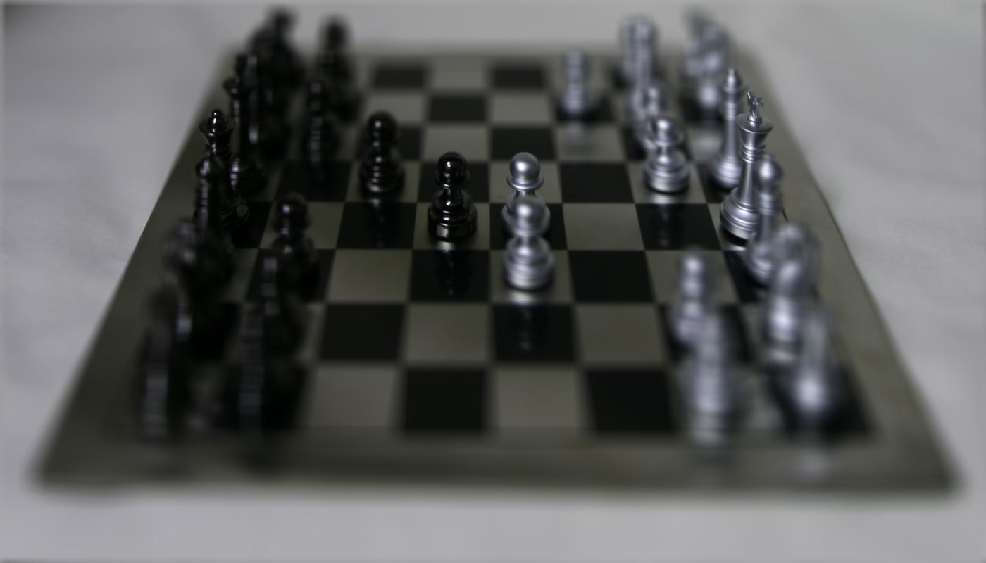
We noticed that the chess dataset was in a slightly different format than the lego dataset (the values increased rather than decreased across the grid), which meant that we had to edit our to be in that case. For lego, we varied from -3 to 3; for chess we varied it from 0 to 3. This was done over 10 frames for both images.
Previously, we included all 289 images in our averaging, but each was shifted. To perform aperture adjustment, no shifting is needed. However, we now only include a subset of all 289 images in our averaging.
The hyperparameter we vary here is . Specifically, we include the image at in our average if . We experimented with other inclusion conditions (L1 norm instead of L2, as well as a square window) but found that the L2 condition generated the most natural looking results.
Varying from 0 to 12 over 13 frames yielded the following gifs:
In lego, the point of focus is the middle figure’s sword — notice how that never becomes blurry. In chess the point of focus appears to be the silver pawn in the third row from the right.
It was fascinating to see that simply averaging several images could recreate cool effects like these. I don’t think we thought this was possible before.
Traditionally when trying to resize an image in one dimension, we stretch or compress it, leading to odd artifacts. Seam carving solves this issue by instead strategically removing “seams” (a path across the image) of low importance. Doing this repeatedly results in an image with reduced dimensions but with the key subjects and structures still intact. This is largely a reimplementation of the ideas in Seam Carving for Content-Aware Image Resizing.
To formally define what it means for a seam to have “low importance” (henceforth referred to as “energy”), we need some metric of the energy of each pixel. The seam of lowest energy, then, is the path across the image with the lowest total energy. The energy of a pixel at position is defined as:
We can compute as the principal square root of
where is the color channel of the entire image. A similar calculation can be made for .
Given the energy of each pixel, our task is now to determine the seam across the image with the lowest total energy. Our implementation assumes that seams are vertical; that is, that they are a path from the top of an image to the bottom, with precisely one seam per row, and with each consecutive pixel’s column varying from the previous by at most 1. In order to determine horizontal seams, we simply transpose our image before searching for seams and compressing.
In order to do this, we compute the cumulative minimum energy for all possible pixels:
The value of for each pixel can be computed using dynamic programming. (Note, here our notation indexes into an image as , but in code this is ). Then, the pixel with the lowest in the last row is the end of the seam with the lowest total energy. To find the rest of the seam, we backtrack our way across the image.
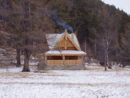
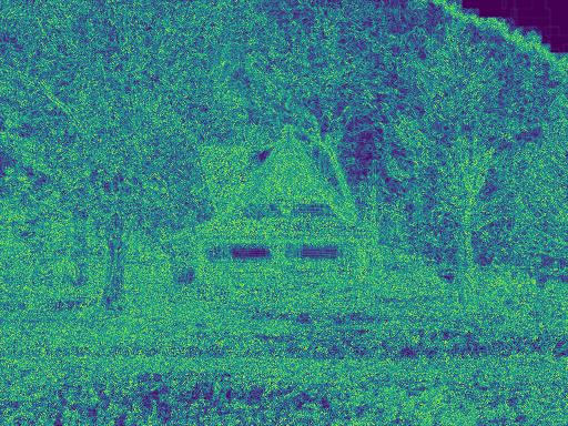
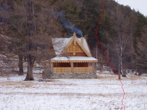
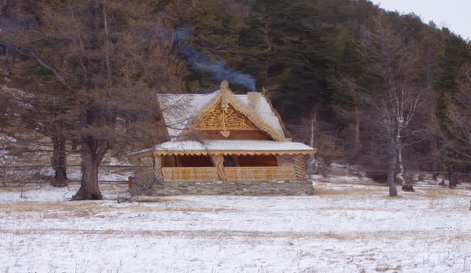
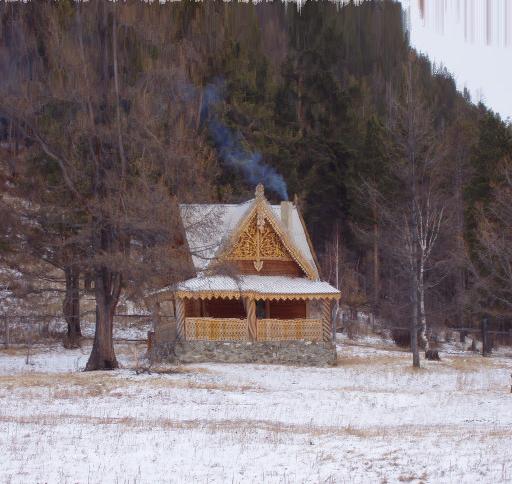
In order to remove the seam, we can create a boolean mask with 0s in the positions of the seam and 1s elsewhere, and call the image with that mask applied. Here is an example provided in the spec (cabin) along with its energy map, and the first vertical seam to be removed:
Removing seams repeatedly can resize our image! Below, we present several images, along with their resized versions using seam carving.
| Name and Action | Original | Resized |
|---|---|---|
cabin, horizontal, 200px |
|
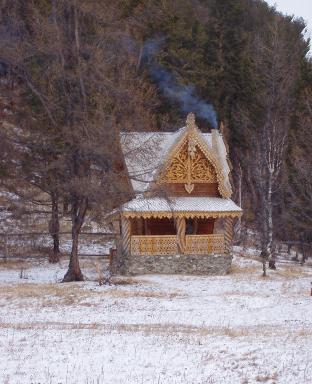 |
cabin, vertical, 150px |
|
 |
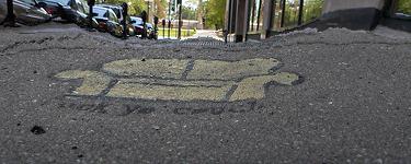
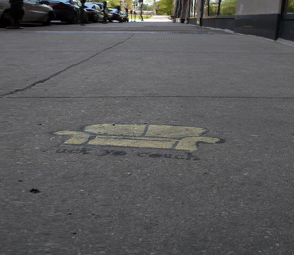
sidewalk, vertical, 350px |
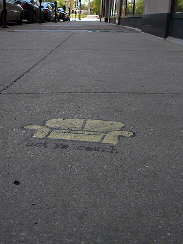 |
 |
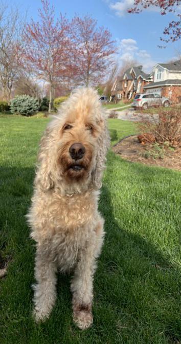
junior, horizontal, 150px |
 |
 |
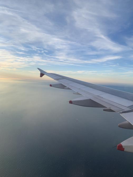
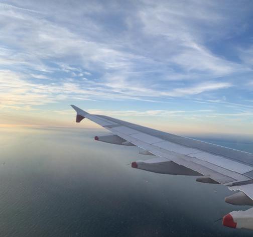
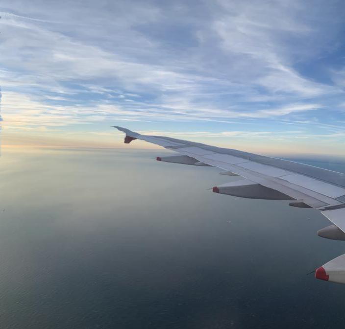
plane, vertical, 200px |
 |
 |
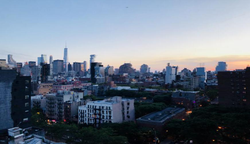
nyc, horizontal, 200px |
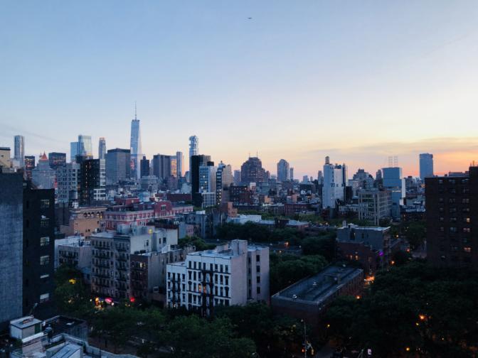 |
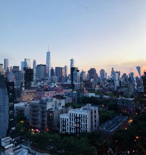 |
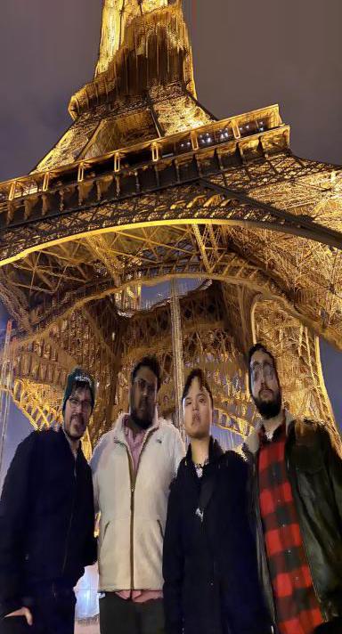
eiffel, vertical, 200px |
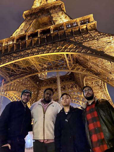 |
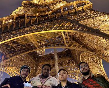 |
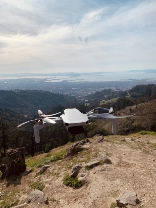
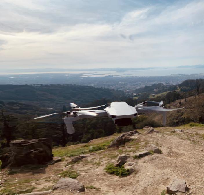
drone, vertical, 200px |
 |
 |
I consider the junior and eiffel examples to be somewhat of a failure. For junior, it deformed the structure of the beloved puppy, and one of the houses in the background is quite deformed. In the eiffel example it got rid of all of our bodies (though we’re probably less important than the Eiffel Tower, so it’s fine), but it also created some deformations towards the top of the tower. Overall, the simple energy function produces some quite satisfying results.
Just like we could remove seams to decrease the width or height of an image, we can also add seams to increase the width or height. A naive implementation of this would determine the lowest energy seam, and duplicate it, and repeat this process times. The issue with this, however, is that it’s likely that the same seam will be duplicated times, resulting in undesirable artifacts.
Instead, we first specify in advance the number of seams that we want to insert. We then remove seams from the original image, while keeping track of which seams were removed. We then duplicate each of those removed seams, giving us an expanded image with some of the least “important” information duplicated.
Again, we present a table of results.
| Name and Action | Original | Resized |
|---|---|---|
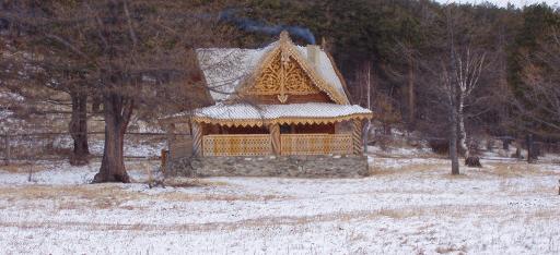
cabin, horizontal, 150px |
|
 |
cabin, vertical, 100px |
|
 |
sidewalk, horizontal, 200px |
|
 |
junior, horizontal, 150px |
|
 |
plane, horizontal, 200px |
|
 |
nyc, horizontal, 200px |
|
 |
eiffel, vertical, 200px |
|
 |
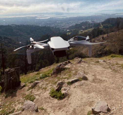
drone, horizontal, 200px |
|
 |
Again, the cabin, sidewalk, plane, nyc, and drone examples largely worked, with some small artifacts. The eiffel example is pretty bad (even worse than the result of the seam removal), and poor junior looks awkwardly stretched.
Seam removal/insertion is a fascinating application of dynamic programming. The results largely turned out well.
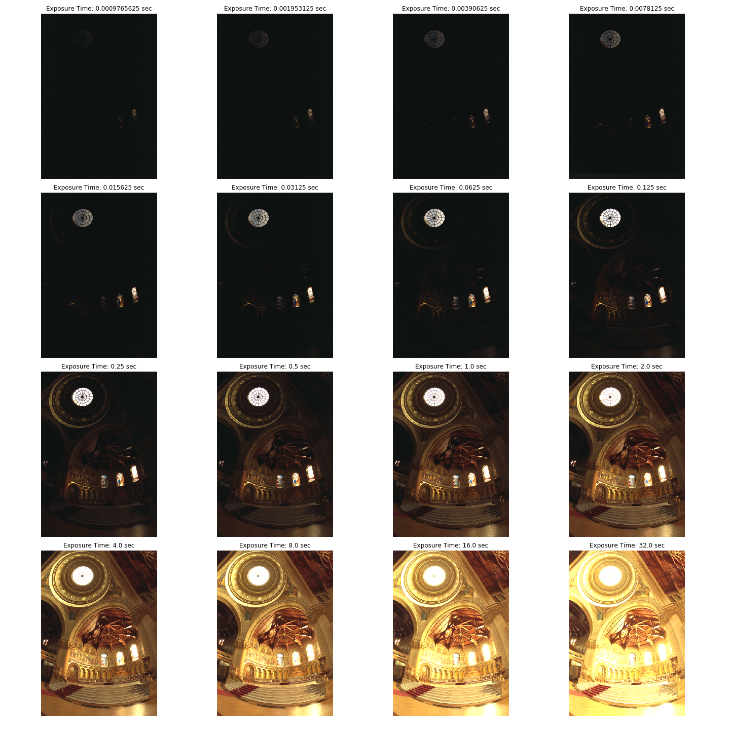
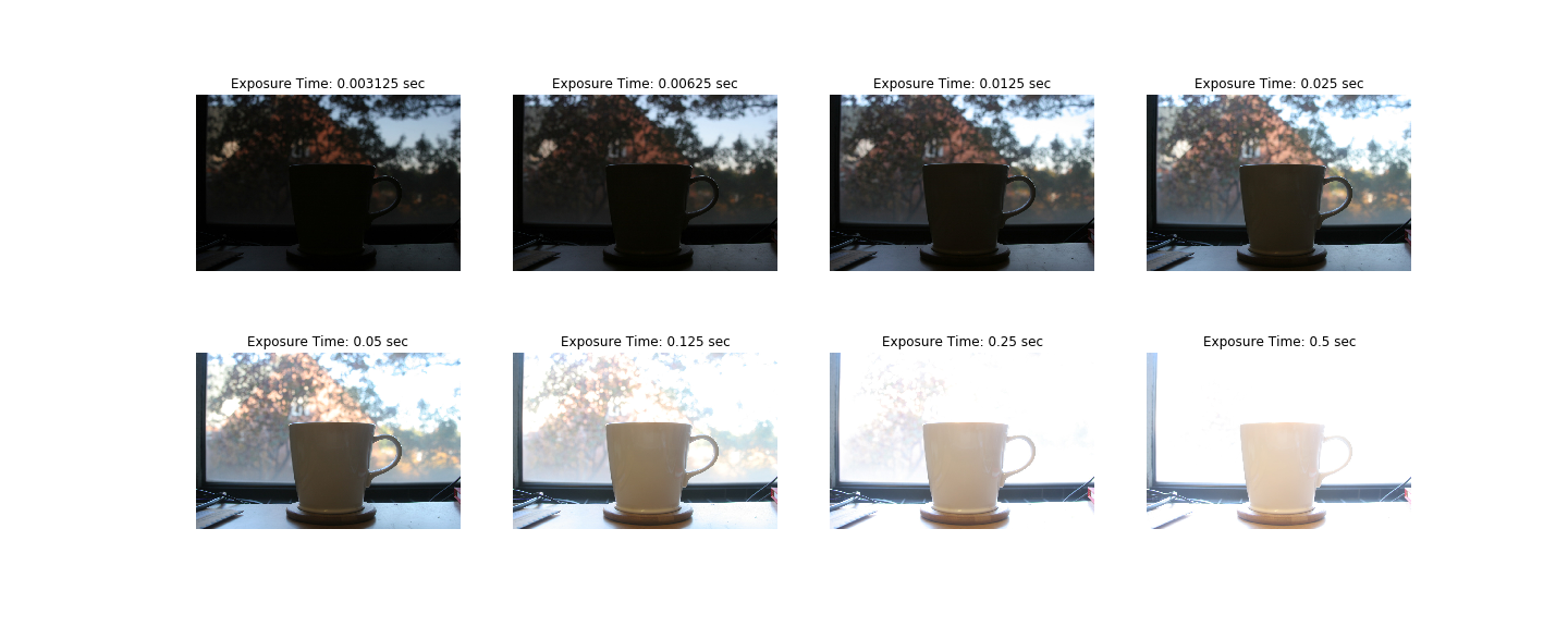
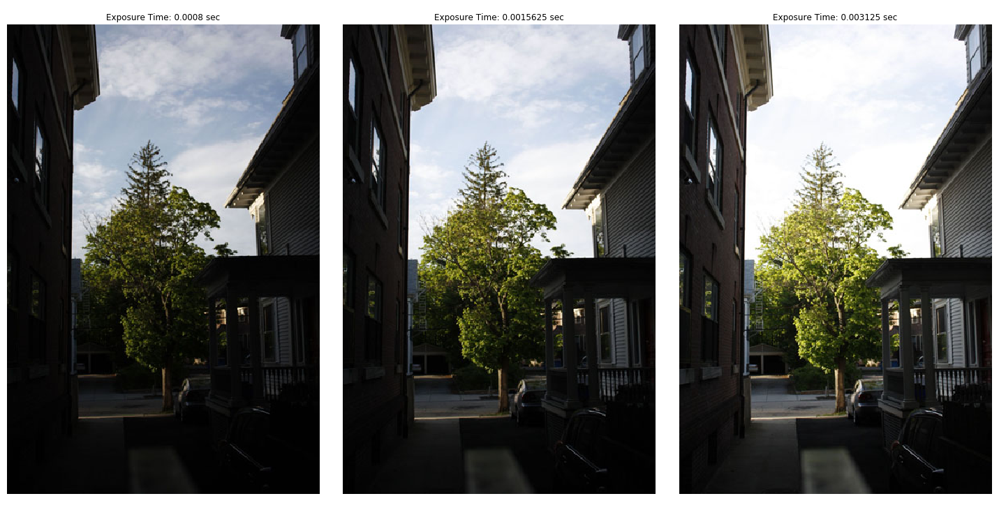
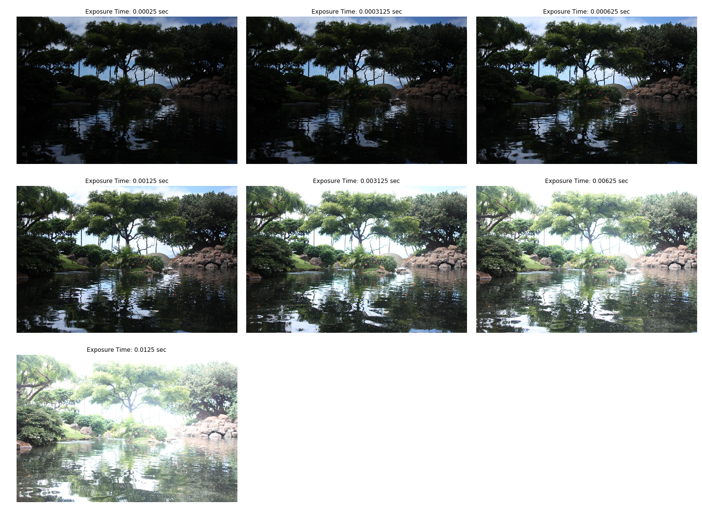
Cameras are, generally, unable to capture the full dynamic range of the world they capture. Most images of a scene with a large dynamic range (both very dark and very bright parts) results in either a partially under-exposed image or a partially over-exposed image. HDR imaging aims to ameliorate this issue by combining information from multiple exposures of the same scene to create an image that more accurately depicts the true dynamic range of the scene.
The HDR task can be split into two main steps:
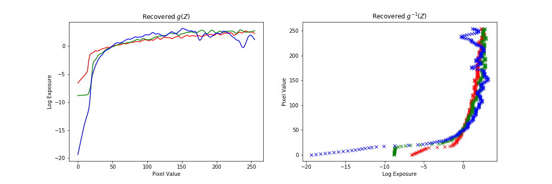
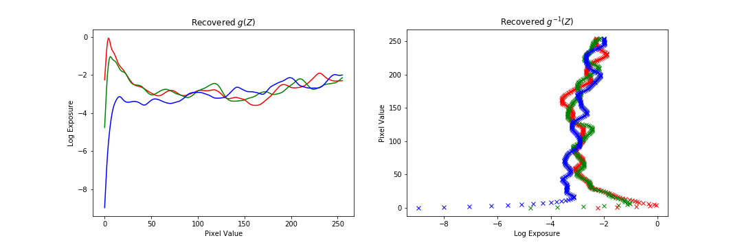
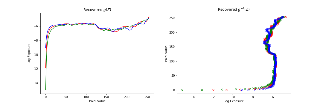
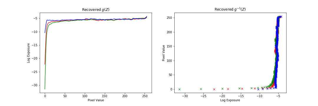
The method we use to build our radiance map is specified in Debevec and Malik 1997. We denote a pixel to be the th pixel in the th image. We can model the value to a be a function of the product of the unknown radiance (which we want to solve for) and the known exposure time : . In general, is some complicated pixel response curve. Rather than solve directly for , we solve for , which maps pixel values to the log of the exposure values: .
Once we have , recovering the radiance map is straightforward. However, solving for is tricky because we know neither nor . But, the key observation is that we know that the value of remains constant across the image sequence. Additionally, as the domain of is pixel values, we only have to solve for values of our function. And, to make the method robust, we add a regularization term on the second derivative of , as we expect to be smooth. Lastly, we weight the contribution of each pixel by a triangle function to account for the fact that very dark and very bright pixel values have more noise and saturation, respectively.
All put together, we can formulate this problem as a weighted, regularized least squares problem (which can be solved as a modified standard least squares problem). We solve for both the function and select radiance values in the least square problem, although we only use the solution to when we construct the overall radiance map. The number of unknowns is thus 256 (values of g) plus the number of pixel values used to solve the equation, and the number of equations is the number of pixels used times the number of exposure images.
Clearly, using all the pixels in the image to solve for is not computationally feasible, so instead we use a subset of values. While the paper says they handpicked values to feed into their solver, we tried to automate this process. We randomly sample pixels, but ensure that we capture the full range of pixel values as well as maximize the variance of values (to try to get a random sample that accurately portrays the data).
The results shown in this description are from computation on the Stanford chapel dataset. Additional examples are shown after the explanation of the entire method.
The Stanford Chapel Dataset:
And the results of the recovered mapping:
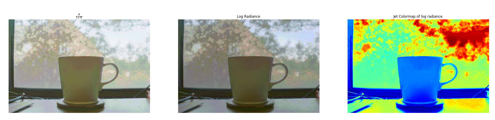
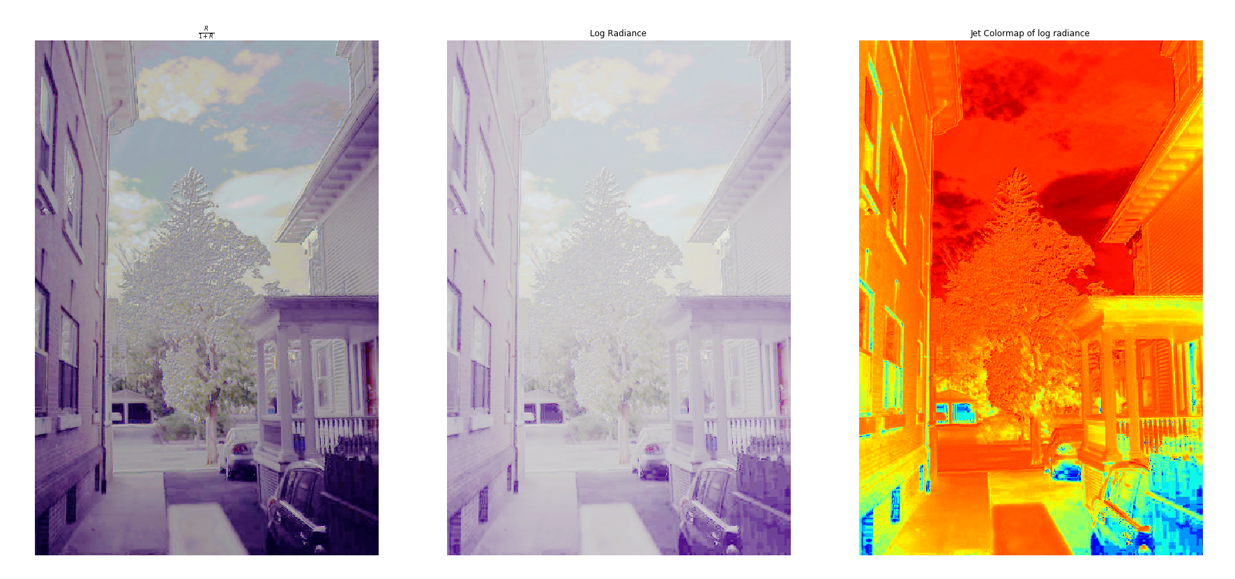
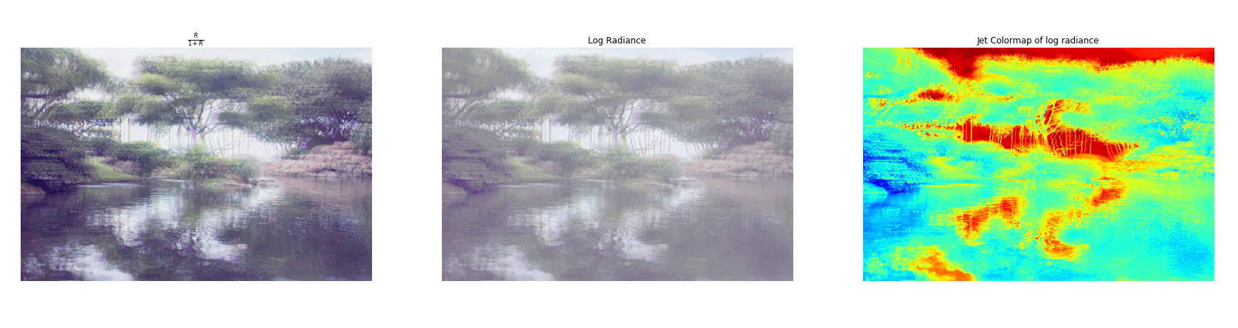
Once we have a radiance map of the image, the next step is to convert this radiance map back into a viewable image that preserves the details of the radiance map. This can be achieved via two methods: a simple global tone mapping, or a more sophisticated local tone mapping method. Examples of global tone mapped radiance maps are and . These two mappings, as well as a “heatmap” visualization, are shown below.
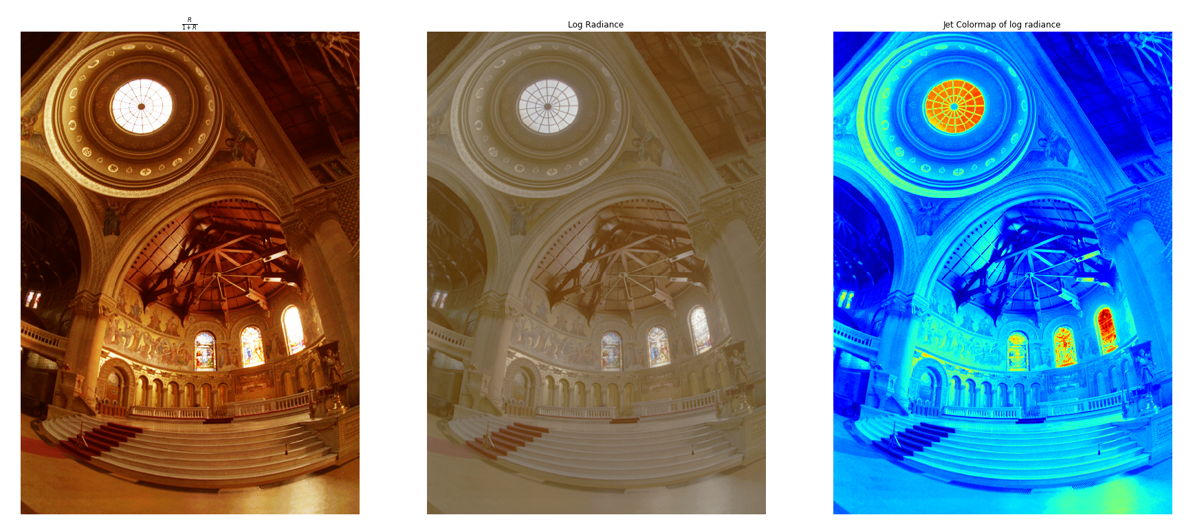
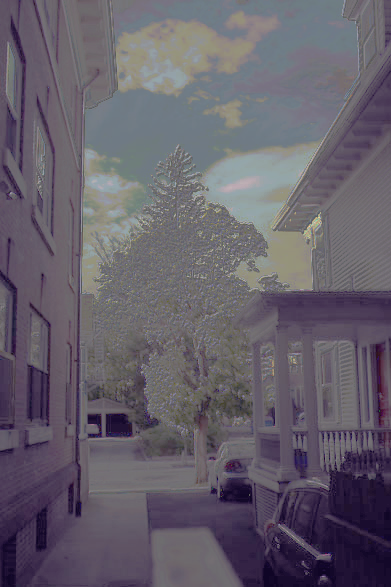
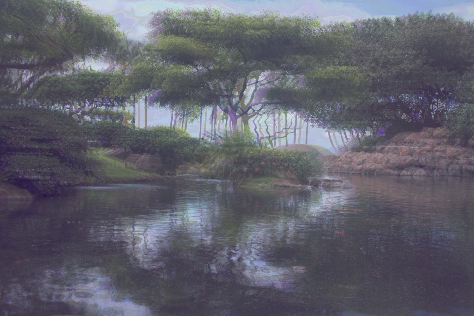
However, we can do better than a global tone map via a local method. The method done here is a simplified version of Durand 2002. The idea here is to use a bilateral filter, a non-linear local filter. The expression of the output for a pixel is
Where is the image intensity at pixel , is a spatial gaussian, is a intensity gaussian, is a normalization factor, and is a neighborhood determined by the standard deviation of the spatial gaussian. What this weighting achieves is a robust, edge-preserving filter, which helps us decompose our HDR image into a base layer and detail layer.
The way this filter is used to create our HDR image from our radiance map is as follows:
With the linear RGB radiance map as input
Apply an offset and a scale to the base:
The offset is such that the maximum intensity of the base is 1
The scale is set so that the output base has stops of dynamic range
Apply gamma transformation:
The result of this local tone map on the chapel, with and :
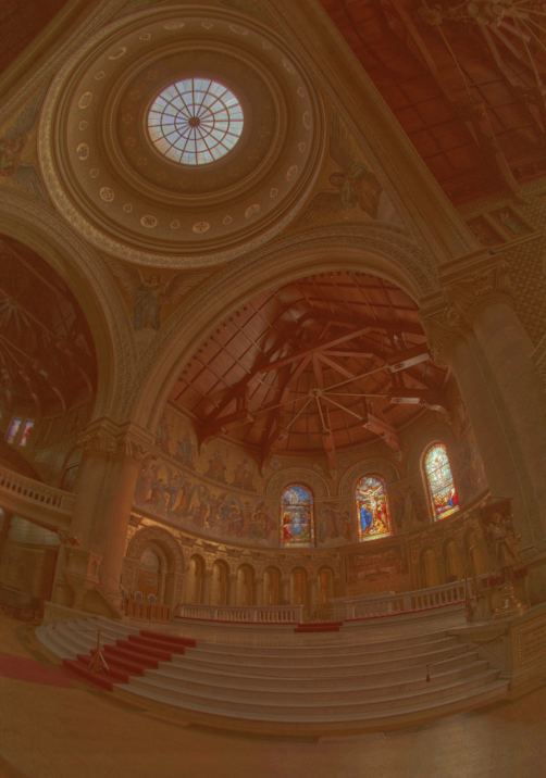
The following are additional results run on the data provided. The results are ok, but in general not as good as the chapel because of the data itself. Either there were not enough exposure times in the dataset, or the alignment was slightly off. Also, personally, I am not a big fan of the radiance map construction method as there are many parameters (number of data points, strength of regularization) that require tuning for each image to get a good result. Additionally, for some images the regularization far out weighed the data consistency term, which leads me to question how much of the mapping construction comes from the data versus our prior.

This was one of our favorite classes at Berkeley. Thank you so much Prof. Efros and the GSIs!