Final Project

Part 1: Seam Carving

Have you ever seen an image on the internet that you wanted to resize? I, for one, have come across several photos that I'd like to be my wallpaper, but they're too small! So they come up really grainy when they get blown up to fit the higher resolution. Or, what if you had a rectangular picture that you wanted to be square? Well, your computer will probably squeeze it and make it end up looking really weird.

In 2007, Shai Avidan and Ariel Shamir came up with a cool idea: what if, when resizing an image, you just remove certain parts of it until you get the size you want? Their key idea was their choice in parts that they removed: they chose to remove parts that were the least noticeable if removed, or as they put it, had the lowest energy. To ensure that things still looked ok they, they ensured that only a connected line of pixels could be removed; they referred to this as a "seam". Thus, their method became known as seam carving, and became immortalized in their seminal paper.

1.1 Seam Removal

In order to remove the seams, we first need to decide how to give "energy" to each pixel. The simplest choice is to simply use a Derivative filter on the image to grab the sharp edges, then take the magnitude of the resulting gradient. This is what they chose to use in the paper as a baseline. It is defined mathematically as:

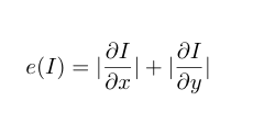
To figure out which seam to remove, we can utilize the following Dynamic Programming approach, where e(.,.) refers to the energy image, and E[i,j] holds the lowest seam energy (so far) that we can use to reach pixel (i,j) from the top:

1. For the first row, E[i,j] = e[i,j]
2. For all subsequent rows, E[i,j] = e[i,j] + min{E[i-1,j-1], E[i-1,j], E[i-1,j+1]}
3. Once at the bottom, find the minimum value of E for the bottom row, this represents the ending point of the lowest energy seam.
4. Backtrack in your path until you recover the seam.

Once we have this seam, we can now remove it from the image. Note that this removes a vertical seam, thus reducing the width. We can repeat this process as many times as we would like to get the desired width. To change the height, we can just transpose the image and repeat the same process.

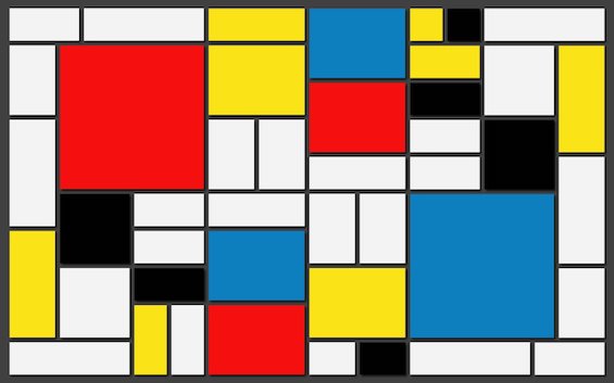
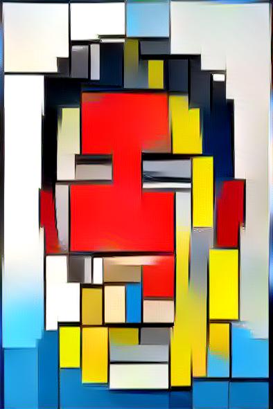
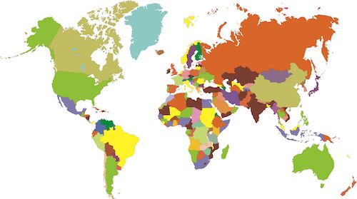
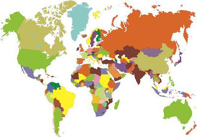
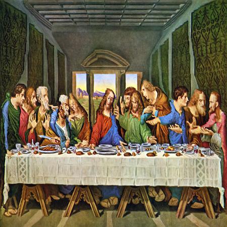
Below, you can see an example of two different energy functions I used: the standard Derivative filter, and also the smoothed Derivative of Gaussians filter. Interestingly, you can see that the non-smoothed filter did better. Why? I think it's because removing seams creates unnatural edges, and smoothing allows us to ignore these. (Note the top of the left tower).

Orignal Image	Derivative Filter	DoG Filter

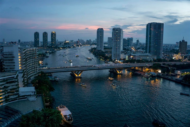
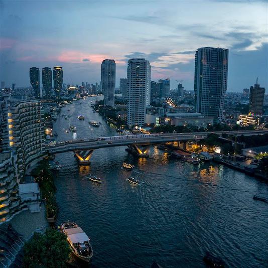
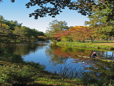
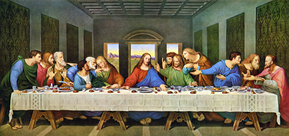
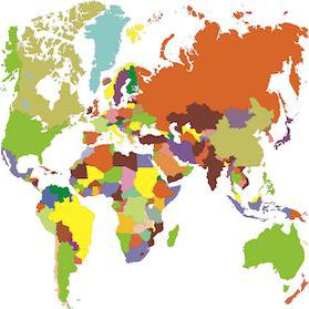
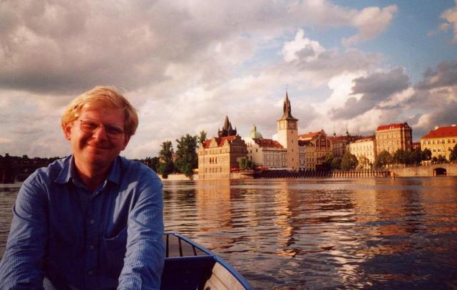
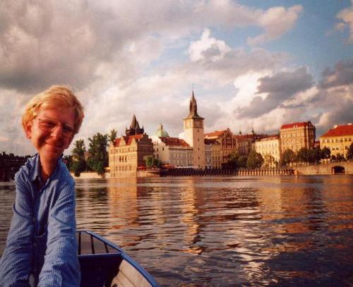
Below, you can see more results for other images.

Orignal Image	Seam Carved

1.2 Failures

Not all of the examples worked too well, If there's too much content along a certain direction and we choose to carve that way, it is forced to remove some important information, leaving us with weird looking pictures.

Orignal Image	Seam Carved

1.3 Seam Insertion

What if we want to increase the resolution? Well, we can just reverse the process of carving. Say we want to increase the resolution by n. All we have to do is find the first n seams we would normally remove, and instead of removing them, add them back to the image. But this would create stretches of repetitive pixels, so instead, we place a new seam in the place of the supposed-to-be-removed one, shift the pixels it overrides to the right, then set its value to be the average of the seams on either side of it.

Below, you can see an example of where I extended some images:

Orignal Image	Seam Inserted

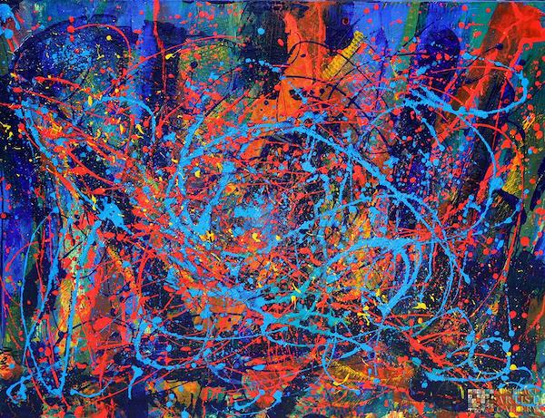
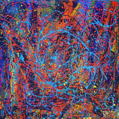
1.4 Deleting Objects

We can actually leverage these two tools now to delete objects from a photo! To do this, we now take in a mask over the part of the image we wish to delete. Then, we aritifically drive the energy values for that area to negative infinity, and then do seam carving for the width of the mask number of iterations. The artifically negative values will force seam carving to delete what we want. Then, to get it back to normal, we just do seam insertion back to the original resolution!

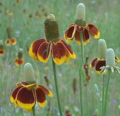
Here are some examples of deletion. As you can see, for something small like the man, it works nicely, but for large parts of the image, it doesn't work as nice as it creates harsh edges

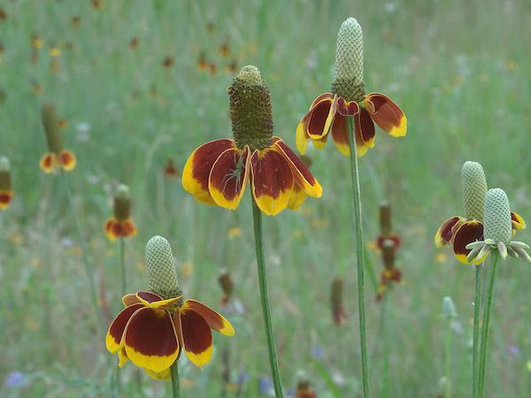
Man Removed	Flower Removed

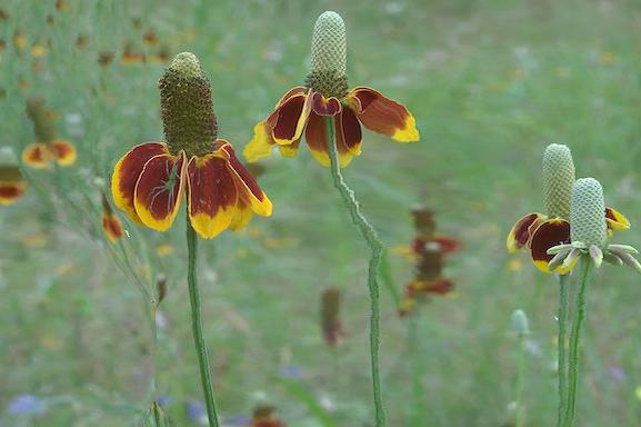
Part 2: Neural Style Transfer

I did this project since it was the coolest result I saw in the class. In 2015, Gatys et. al decided to look at the information contained within a Convolutional Neural Network and realize that they can leverage that information to do something amazing: take one image and transform it into the style of another! Their seminal work launched a new area in computer vision research, with significant imporvements in speed and quality made since then.

2.1 How It's Done

How did they do this? First, they broke up an image into 2 components: content and style. In order to transfer the style of one image into the content of the other, they first had to extract the content and style information of these images. To do this, they took a pretrained Convolutional Neural Network, VGG-19, one of the densest networks out there, and looked at the outputs of the neurons in each layer. In a convolutional layer, the layers make use of filters as neurons, which means that each layer encodes some information about regions of the image, instead of each pixel. The lower you are in the network, the lower level the information you get: i.e. you can find information about edges in the lower levels, whereas higher levels are able to understand more abstract things such as what you are looking at.

So, instead of training a network to do something, we are instead training an image to be as good as possible. I call tis the generated image. Thus, in their approach, they define two kinds of loss: content and style.

1. Content Loss: The squared difference between the outputs of the "content" layers for the content image and the generated image.
2. Style Loss: For this, they took the outputs of the "style" layers, and instead of comparing them directly, utilized their Gram matrices. This is equivalent to the covariance matrix, where the features are the layers: take the inner product of each layer with each other. Then, we compute the squared difference between these resulting Gram matrices for the style and generated images.

Finally, we can get an overall loss, which is a weighted combination of the Content and Style Losses. Gatys suggests using a ratio of 1000:1 for style to content weight. Thus, our optimization formulation is complete: minimize this loss with respect to the generated image. While you could use any descent method to optimize, they chose to go with LBFGS, a quasi-Newton descent method, with a learning rate of 1.

2.2 Hyperparameters

The key to getting this algorithm working effectively is to choose the appropriate hyperparameters. I found that the most important one was choosing which layers should be the "content" layers and which should be "style". The paper suggests to use "conv4_2" as the content layer, and "conv1_1", "conv2_1", "conv3_1", "conv4_1", and "conv5_1" for the style layers. In the same vein as this, the choice of content and style weights were also important as well.

2.3 My Design

I mostly stuck with what Gatys suggested, but made a few adjustments.

1. I still used the pretrained VGG-19 network, and replaced the MaxPooling layers with AvgPooling layers as suggested.
2. Instead of using the SSE for the losses, I used the Mean Squared Error instead, as it is an unbiased estimator.
3. I used the same style layers, but used "conv5_2" for content, as I found that my results were too skewed towards content and not enough to style.
4. To further encourage style, I chose 0.1 for my content weight, and 1000 for my style weight.
5. I trained it for 500 iterations.
6. Instead of initializing my resulting image at some random noise, I initialized it to be the content image. This is because I found that this algorithm was highly susceptible to converging to a local optima with a lot of noise.

2.4 Neckarfront

Here, we can compare the differences between my results on the Neckarfront houses in Germany versus the results obtained by Gatys. You can see the effect of content initialization compared to Gatys' random noise: the houses are more visible as opposed to more intense style transfer. This is especially prevalent in expressionist paintings such as Kandinsky's.

Style	Style Image	Gatys	Me
Starry Night by Vincent Van Gogh
Femme Nue Assise by Pablo Picasso, 1910
Composition VII by Wassily Kandinsky, 1913
Der Schrei by Edvard Munch, 1893

2.5 Fun Results

Here are more examples of style transfer. I had a lot of fun doing these!

Style	Style Image	Transferred
Starry Night by Vincent Van Gogh
Untitled by Jean-Michel Basquiat, 1982
Girl Before a Mirror by Pablo Picasso, 1932
Piet Mondrian

2.6 Failure Case

Someone requested for me to do a picture of him in the style of his favorite comic, Astérix le Gaulois. It worked alright, but it did show the pitfalls of the style transfer; instead of really transferring the "style" in general of the artist, it's transferring the explicit style of the image we provide. As you can see, in the style photo, the beach is adjacent to the water, so when it transferred, it saw the ground as analagous to the beach and thus tried to paint the sky as the water instead.

Style	Content Image	Style Image	Transferred
Astérix le Gaulois by Albert Uderzo, 1961

Conclusion

Overall, this was a very rewarding final project. I started early, which gave me plenty of time to implement the basic functionality, speed it up, and try some of the bells and whistles. This really came handy when it came to tuning the Neural Style Transfer, which was nice. I was very impressed by the results of both: they are actually very straightforward ideas that don't use fancy tricks, and get very cool results. This was one of the few times in my Berkeley career where I felt proud to show off what I had made!