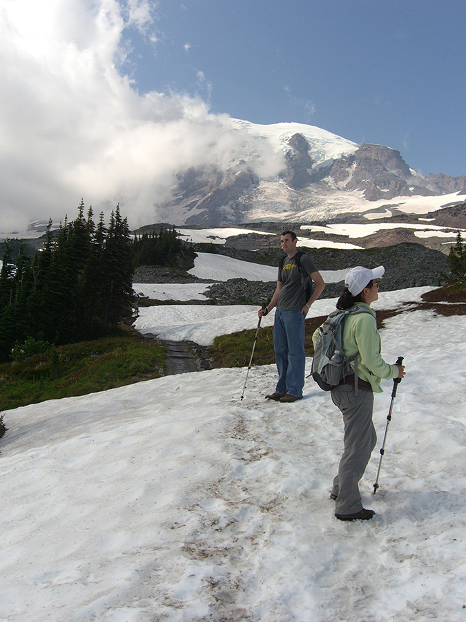
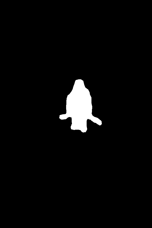
For this project, we want to blend images by preserving the gradient relationships among the pixels in the original image. By dong this, we can blend one source image onto the target image more seamlessly than by simply copy and pasting the source onto the target image. With this way of blending, the source image will take on the color profile of the target image, specifically the pixels that are surrounding the area in which the source image is being placed onto the target image. The crux of this problem is to solve this least squares equation below, or the blending constraint, that solves for the gradient in the masked area of the source image for the new image value to be put in the target image.
To solve the Toy Problem, we use gradient domains to reconstruct the given toy image. To do this, we set the upper left pixel to be equal, and then reconstruct the rest of the image by computing the gradients, in the x and y directional derivatives. We do this by solving the equation above, which will return a solution vector. The output will thus be a reconstructed toy image, with gradients computed on its own with pixel values of the original toy image. Below are the output, with the original toy image on the left, and the reconstructed toy image on the right. The reconstructed image is almost identical to the original.
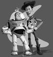

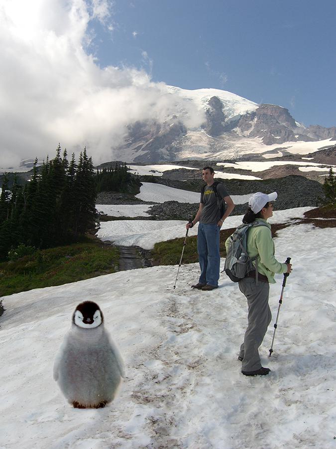
By solving the Least Squares equation above, we were able to reconstruct an image. We will apply the same idea to fill the pixels of the source image into the target image. The target image will essentially be the background that we want to paste our source image into. For any pixels in the background that are unaffected by the pasting of the source image, we just copy the pixel value from the original target image. For pixels that are within the region S, where the object from the source image is to be placed, we solve for the blending constraint. Solving for this will allow us to match the gradients of the target image, so that the object being placed looks less out of place in terms of the color pixel values.
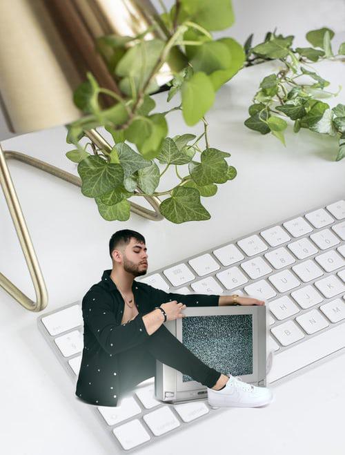
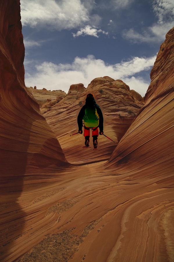
The images of the first example were given in the spec, and the other images following were taken from Unsplashed. For creating masks, I used the Python starter code found here, written by a former student of CS194-26. As for aligning source and target images, I used used the Layering tool in Illustrator to find where the source image aligned the mask created by the starter code, only for the first penguin with hikers blended image. For the two following, I chose pictures of the same size so that they did not have to be rescaled or realigned to be properly blended into the target image.
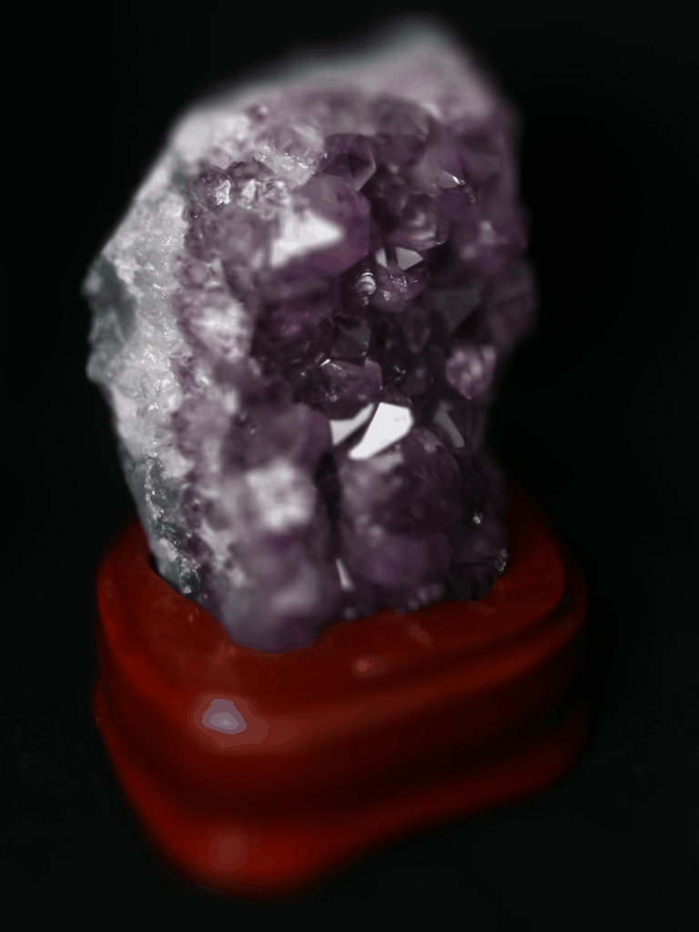
This project is based off the research paper found here. We apply the techniques found in the paper to Stanford Light Field Library's image datasets found here, to demonstrate depth refocusing and aperture adjustment. Each image dataset includes 289 photos taken on a 17x17 grid, with the perspective shifting on the same 2D orthogonal plane. Our task is to manipulate these datasets to mimic taking images with different depths of focus and aperture size.
By averaging all images with different amounts of shift to generate images which focus at different depths. This works because averaging all images without shifting will make objects far away appear sharp, and nearby object appear blurry. So if shift images before performing the average calcuation, we are able to focus objects at different depths, where shifting images such that they align at a certain point simulates focusing on that point. For each image, we compute the x_shift, y_shift = s * (u, v), where x_shift and y_shift are the displace in the x and y direction respectively, and s is a scalar that determines the degree of shift for each image. For the results below, we compute the average shifted image, with s ranging in integer value from 0 to 5. This shifts the focus from top to bottom of the images.
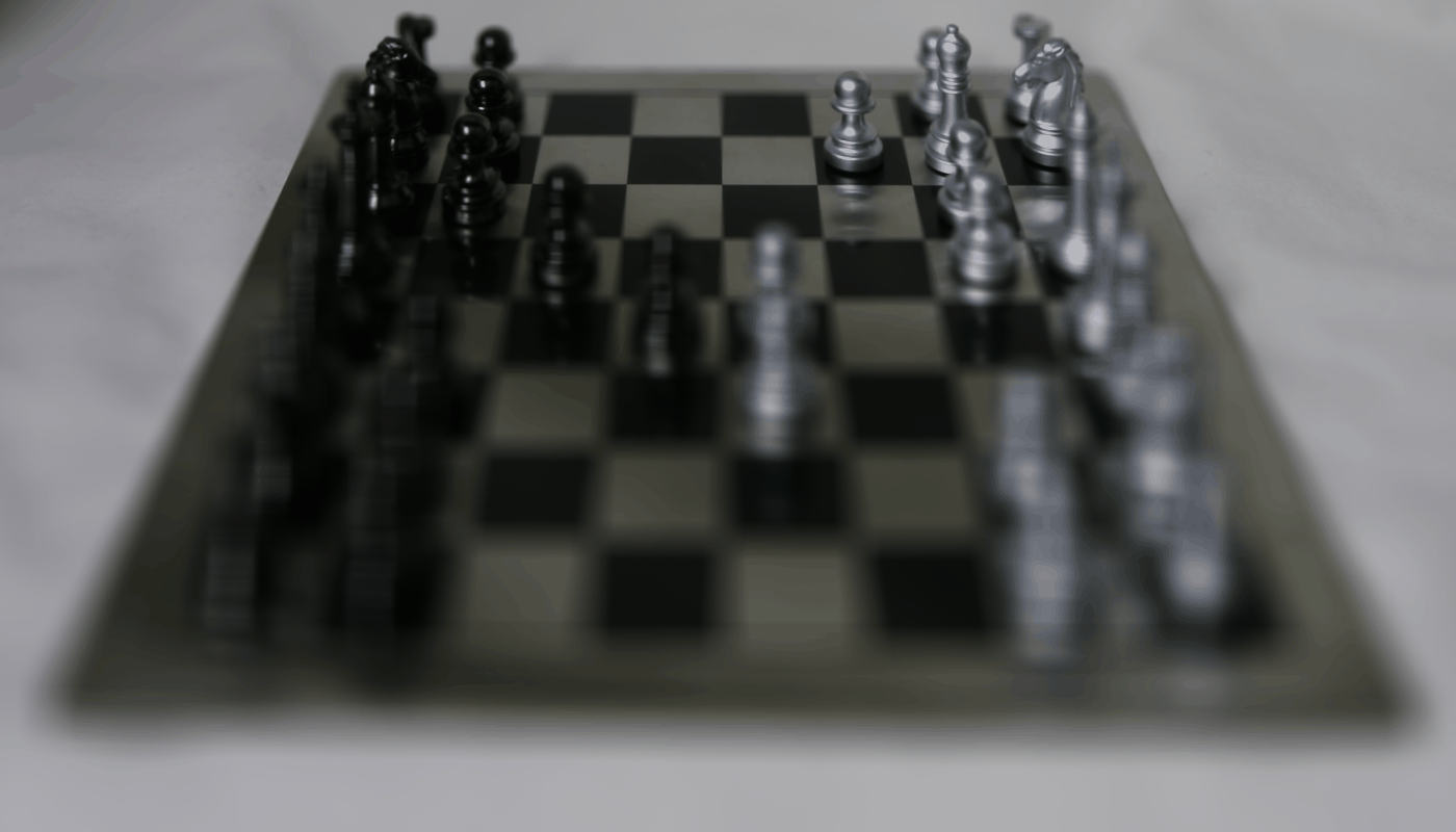
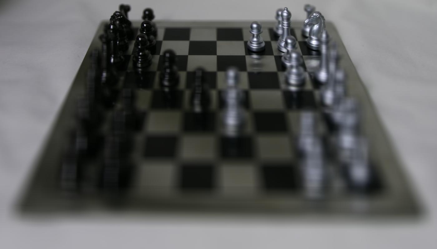
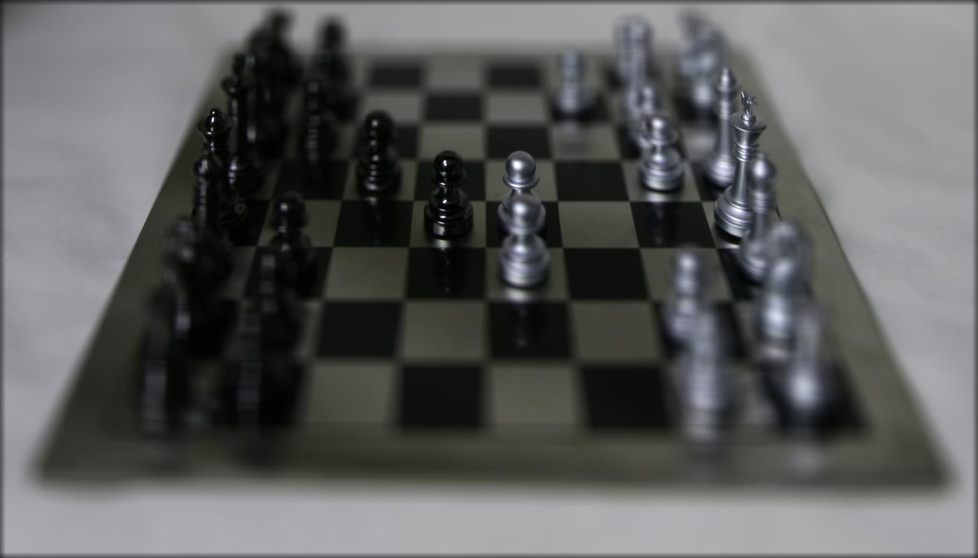
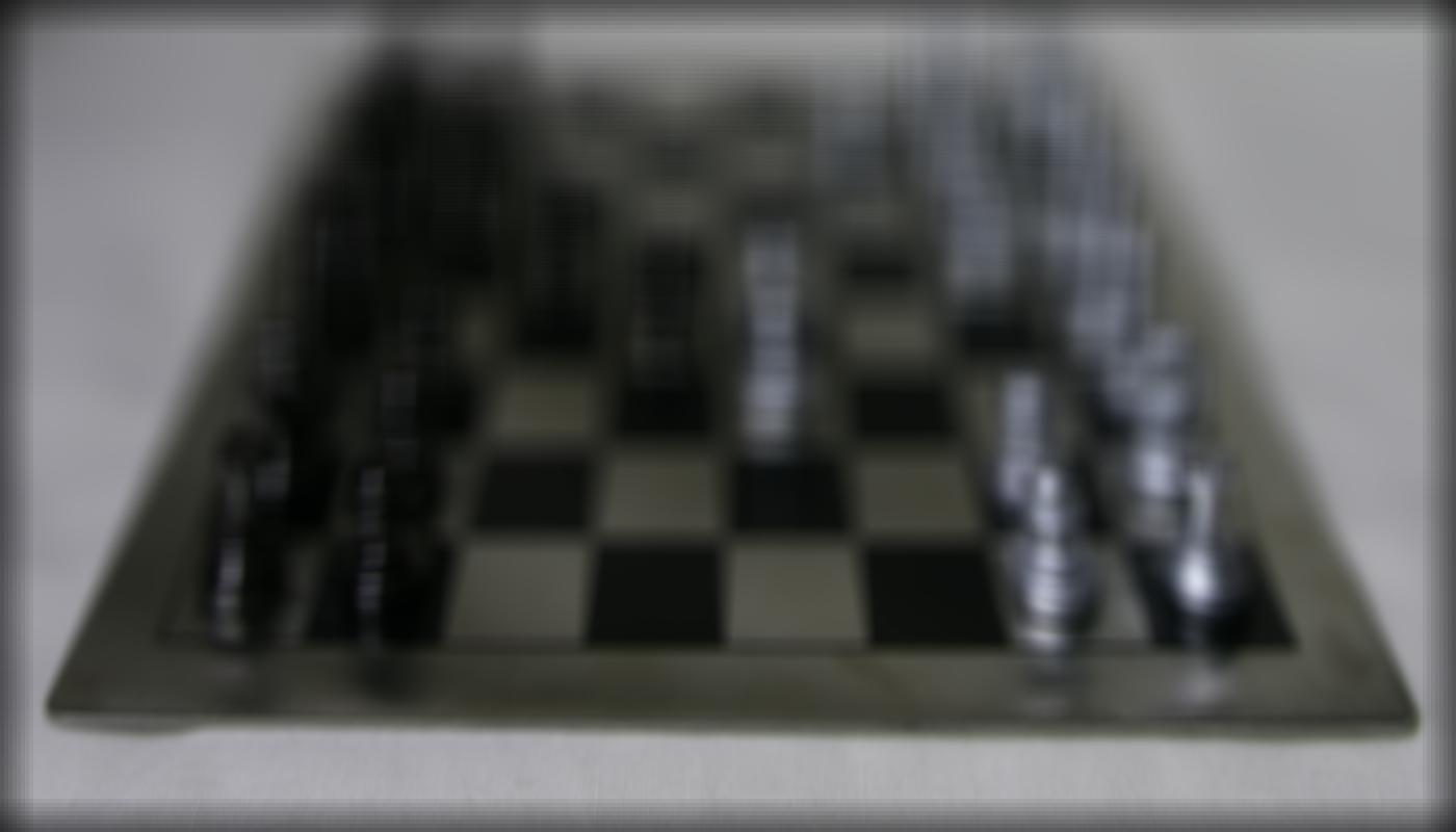
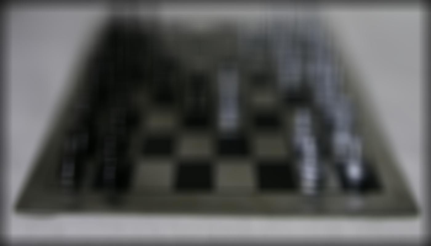
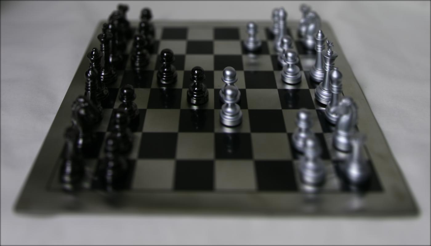
Below are the images that the chess board depth refocusing animation is comprised of, ranging from scalar weight s = 0 to s = 5 from left to right.
To mimic the adjusting of the aperture, we can control the number of images sampled over the grid perpendicular to the optical axis. By averaging a large number of images, we in turn mimic a larger aperture, as a larger aperture would allow for more light rays with different angles to come into the lens. This creates more blur everywhere in the image except where the light rays converge at a point, the point being smaller or more focused when there are more light rays from all directions coming in. By averaging a smaller number, we mimic a smaller aperture, with less data to recreate the image from, much like when we have a smaller aperture in a camera. To pick which images to average, we use a radius r, ranging from 0 to 8. At each iteration, images are included if they are within the camera grid radius will be included.
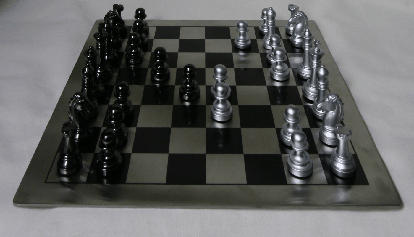

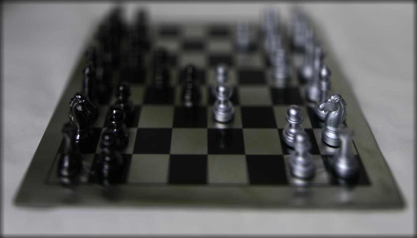
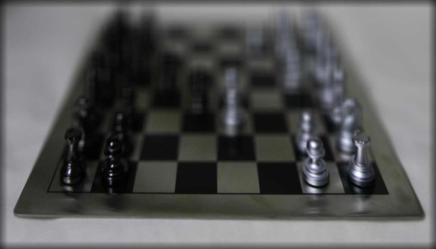
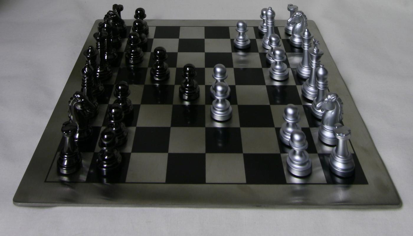
Below are the images that the chess board aperture adjusting animation is comprised of, at radius r = 0, r = 3, r = 5, r = 8, from left to right.


This project helped me better understand depth refocusing and aperture adjustment, and I have never understood it intuitively, only memorizing what the effects of adjusting each of those were. It was cool to relate these results visually, by manipulating these image datasets, versus seeing it through a lens while taking a photo.