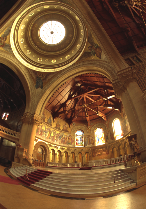
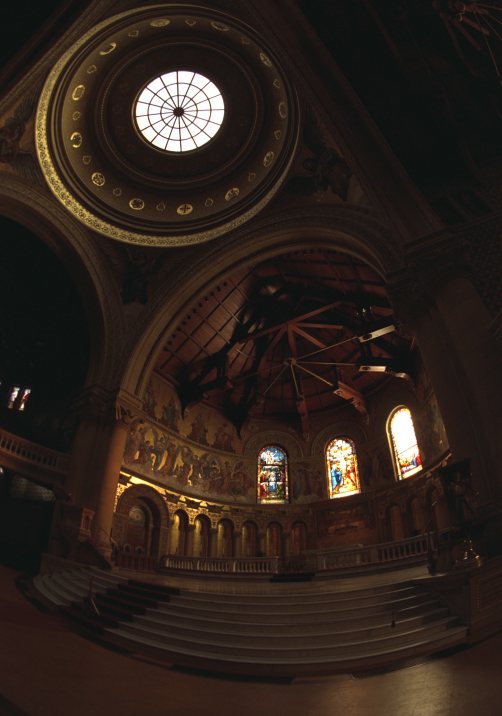
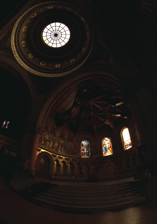
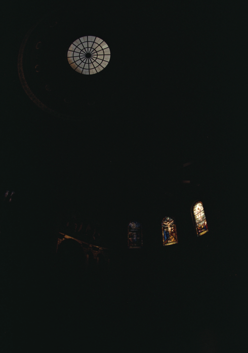
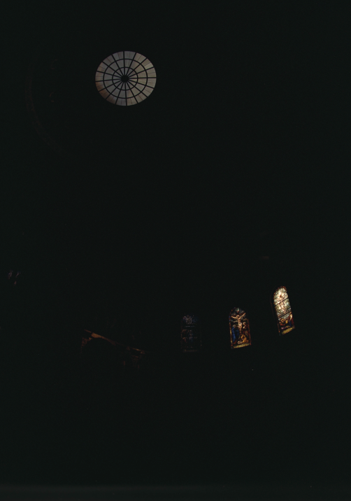
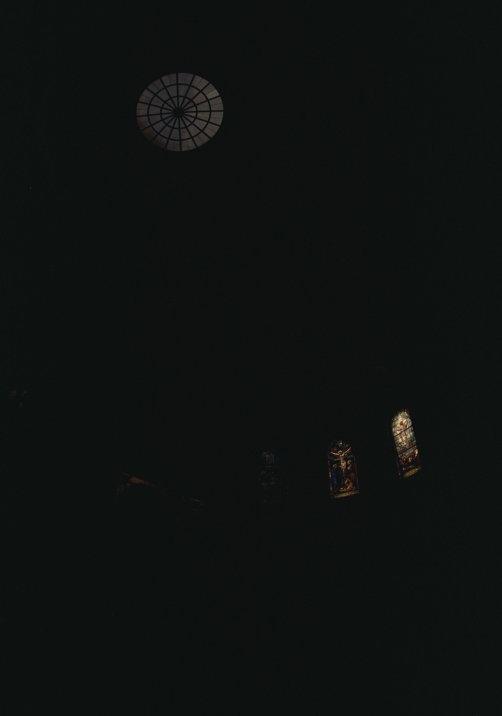
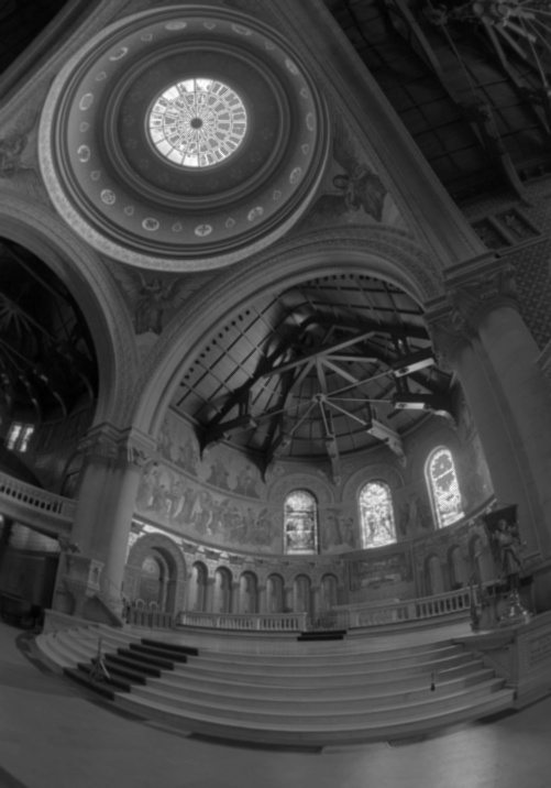
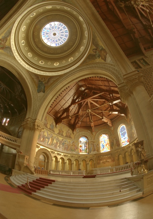
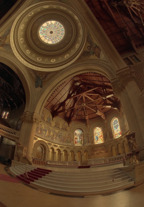
Chapel
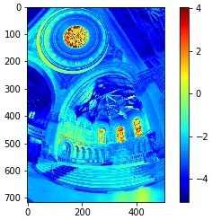
Radiance Map
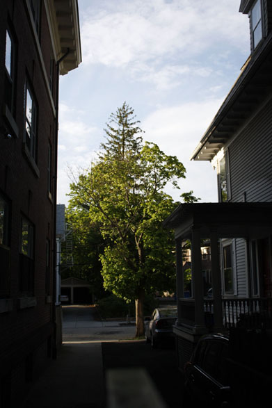
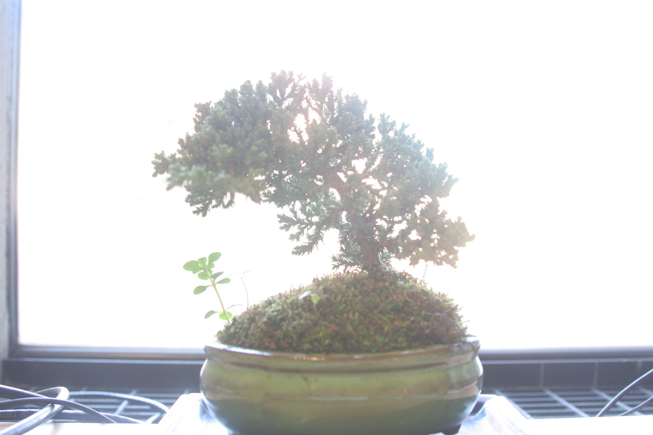
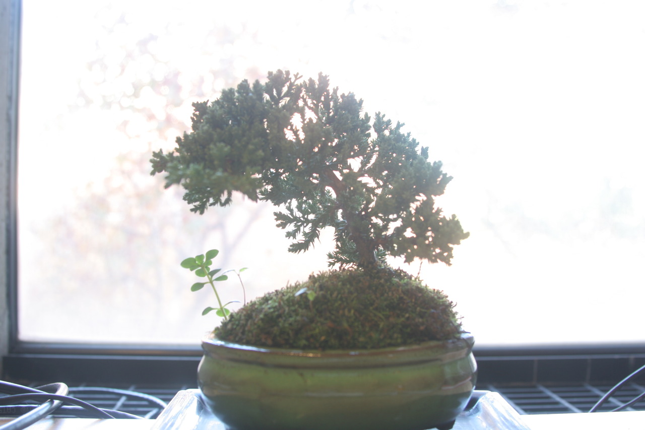
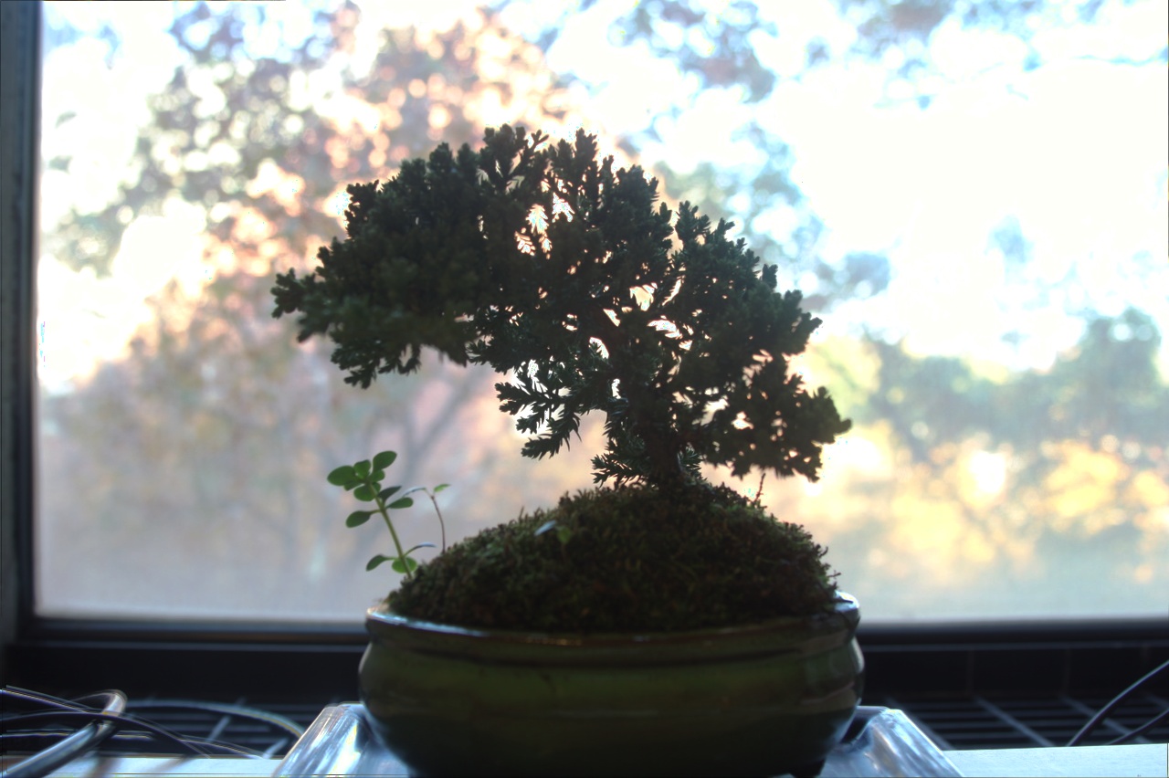
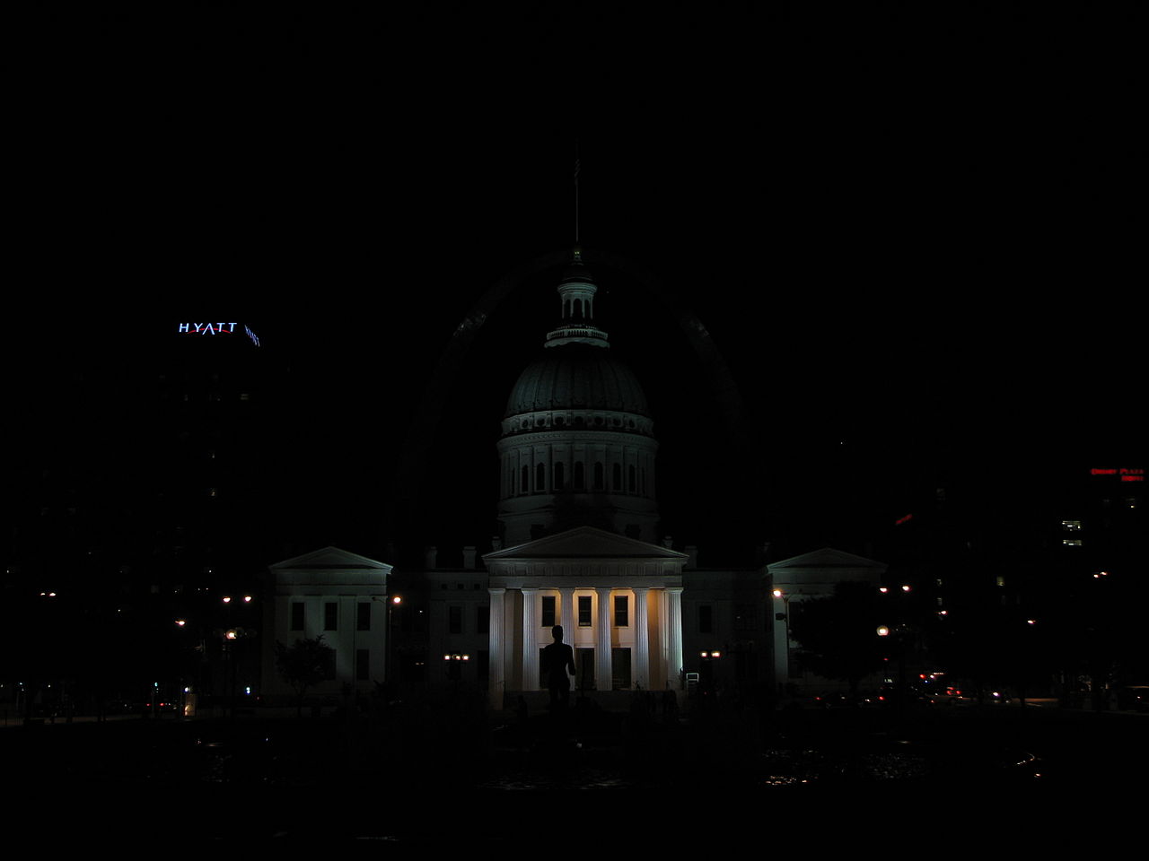
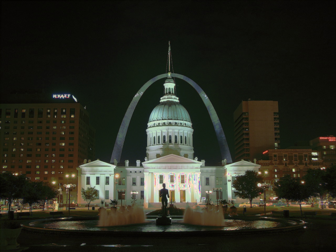
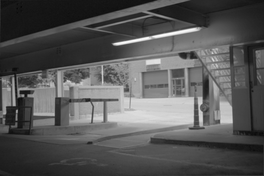
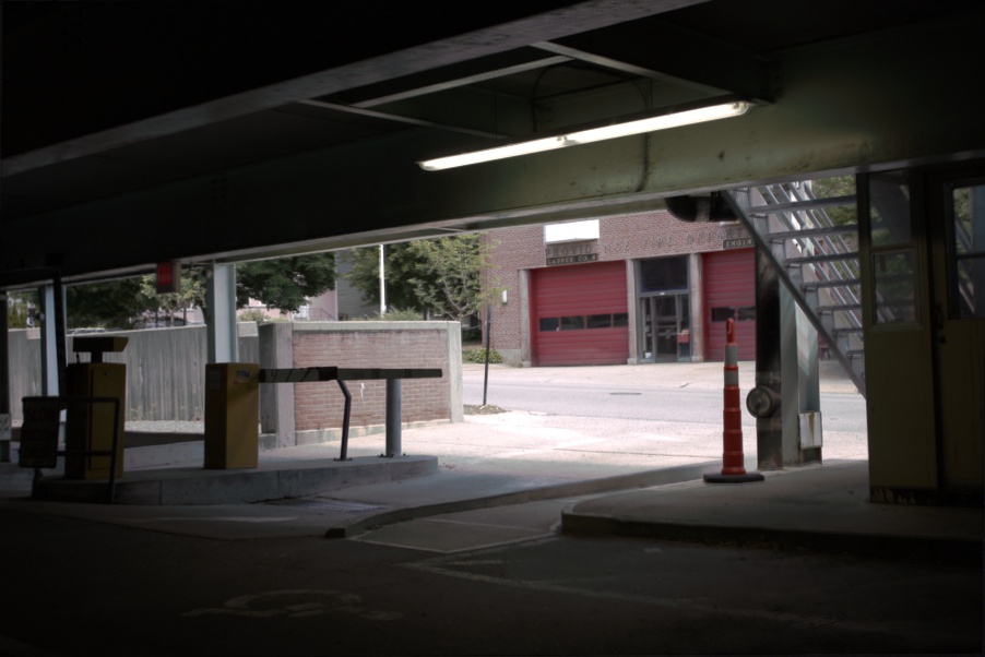
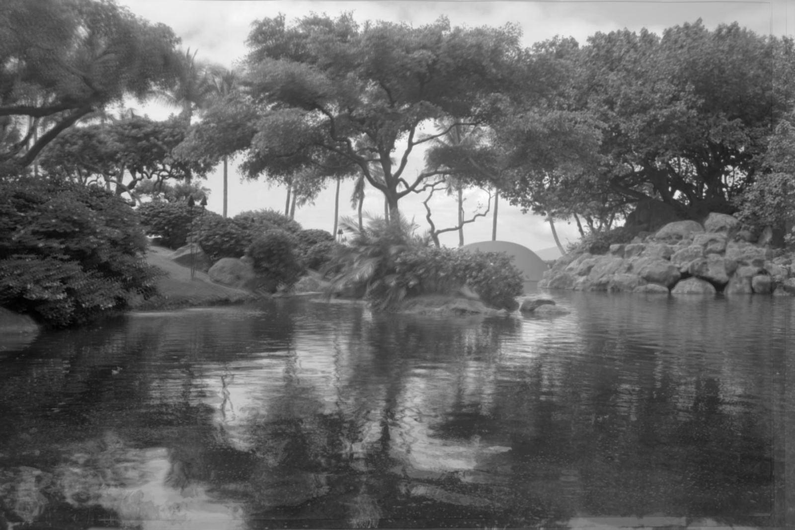
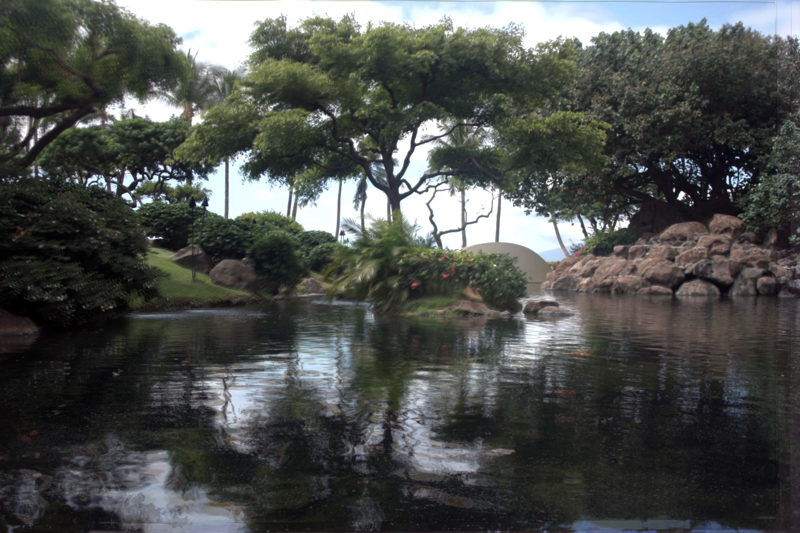
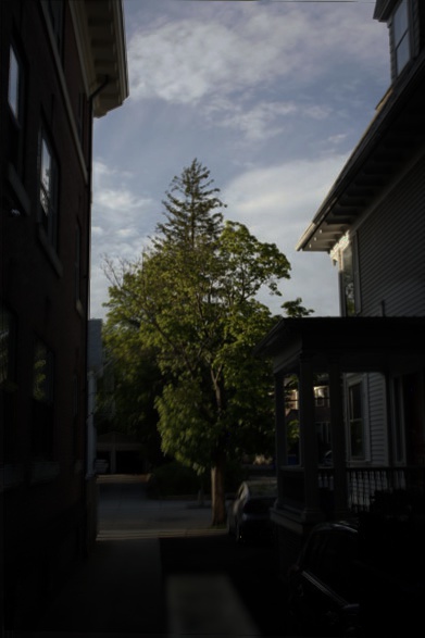
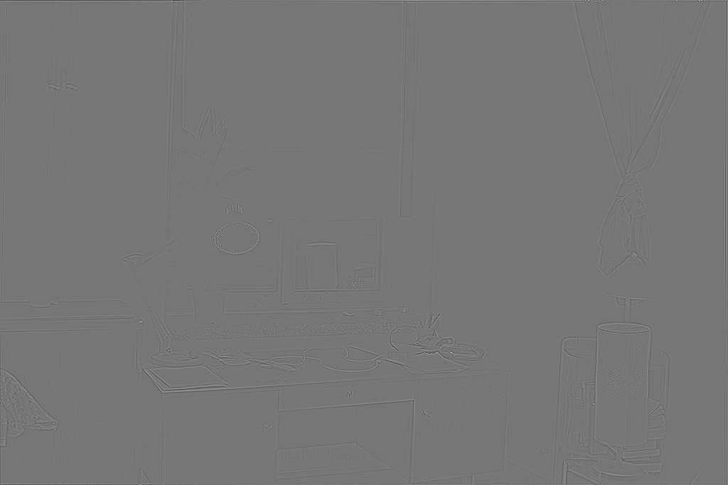
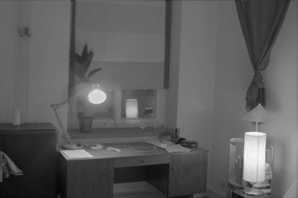
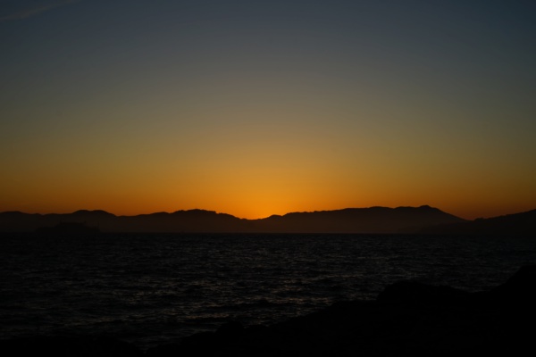
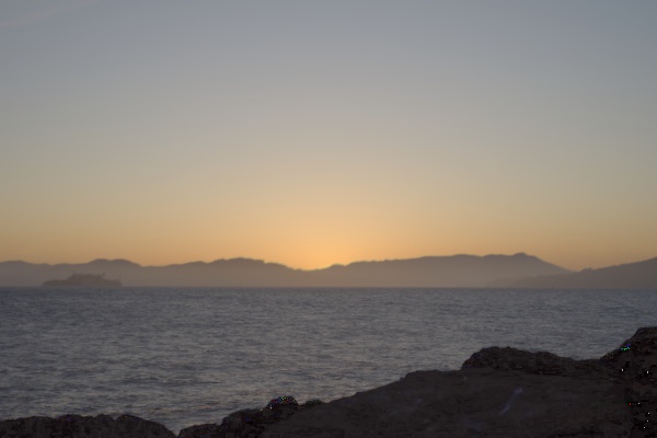
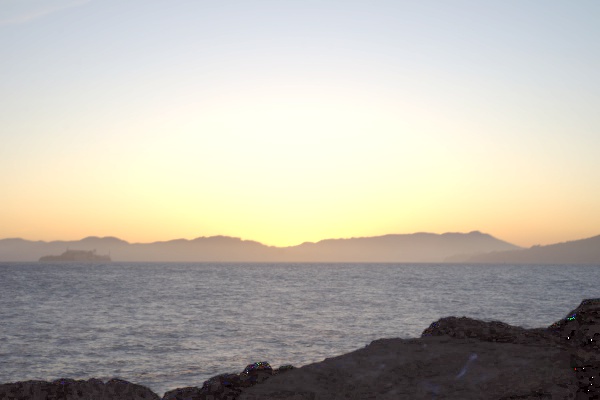
House
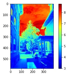
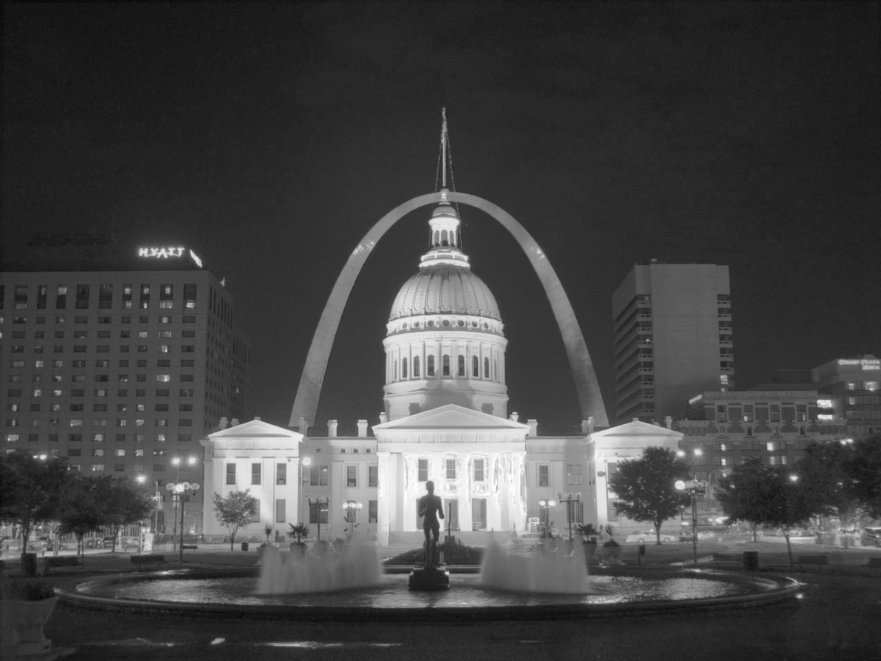
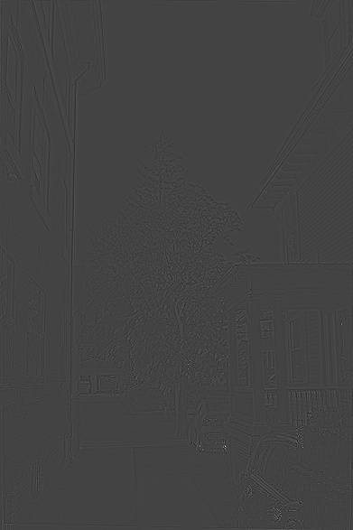
Radiance Map
cs194-26-agf | Chelsea Ye cs194-26-agbThis project attempts to create HDR photos by automatically combining multiple exposures into a single high dynamic range radiance map, and then converting this radiance map to an image suitable for display through tone mapping. The first step of creating radiance maps follows the algorithm presented in the paper by Paul E. Debevec and Jitendra Malik, Recovering High Dynamic Range Radiance Maps from Photographs, and the second step of tone mapping follows the method by Fre ́do Durand and Julie Dorsey, Fast Bilateral Filtering for the Display of High-Dynamic-Range Images.
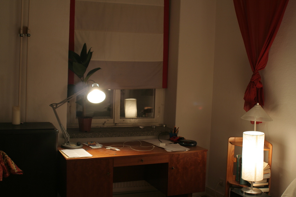
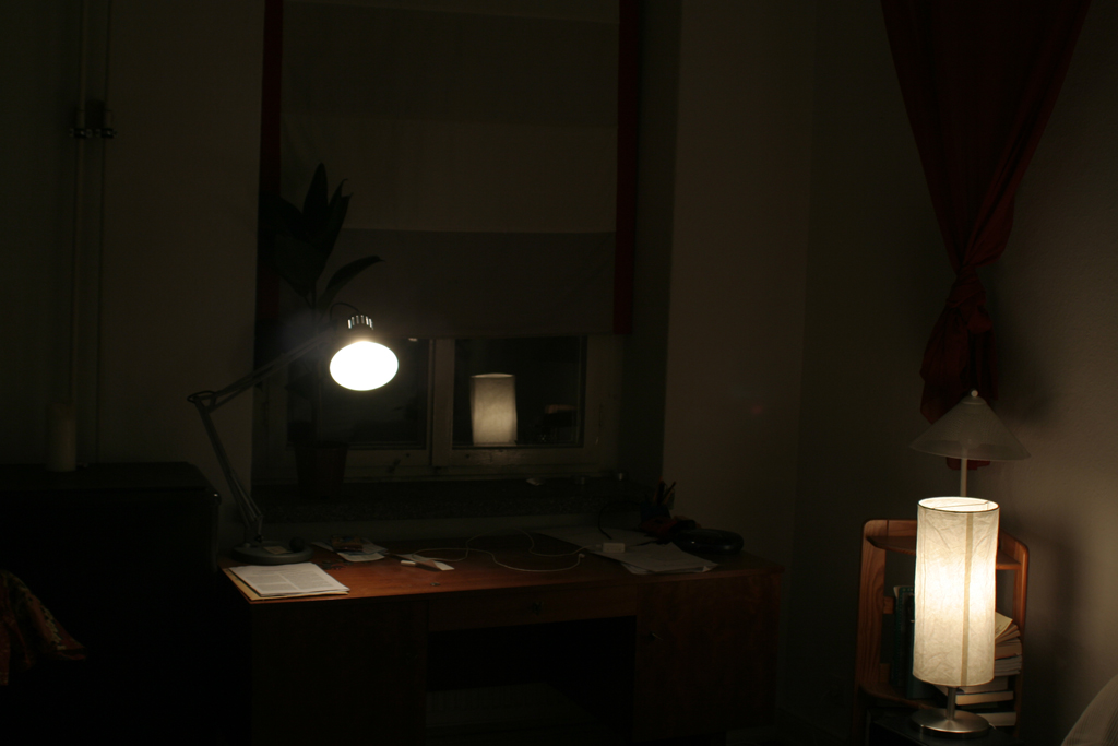
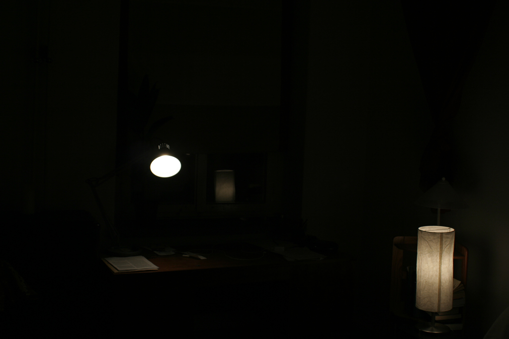
The observed pixel value \(Z_{i j} \) for pixel \(i\) in image \(j\) is a function of unknown scene radiance and known exposure duration: \[Z_{i j} = f (E_i \nabla t_j)\]. \(E_i\) is the unknown radiance and \(\nabla t_j \) is the exposure time at pixel \(i\). Together their product is the exposure at that pixel. And \(f\) is an unknown, complicated pixel response curve. Instead of solving for \(f\), we solve for \(g = ln(f^{-1})\) which maps a discrete pixel value (0 to 255) to the log exposure at that pixel. The function \(g\) can be written as: \[g(Z_{i j}) = ln(E_i) + ln(t_j)\]. Since the scene radiance remains constant across multiple images that we take and we know the exposure time, we can try to solve for \(g\) by setting up a quadratic objective function that we wish to minimize: \[O = \sum_{i=1}^{N} \sum_{j=1}^{P} (g(Z_{i j}) - ln(E_i) - ln(\nabla t_j))^2 + \lambda \sum_{z=1}^{254} g''(z)^2\] where the first term ensures the solution satisfies the previous equation as close as possible and the second term is a smoothing function whose effect we examine below. Having obtained \(g\), we can find the scene radiance by rearanging the above equation: \[ln(E_i) = g(Z_{i j}) - ln(\nabla t_j)\]. During our estimation, we also apply the tent weighting function as suggested in the paper. All the exposures contribute to the final resulting image. However, darker pixels tends to have higher noise and the bright pixels also satuate. Therefore, we give less weighting to those pixels. The formulation of such weighting function as suggested in the paper is: \[ w(z) = \begin{cases} z \text{ for } z \leq 127 \\[.5em] 255 - z \text{ for } z > 127 \end{cases} \]. We show the reference image (one image selected from each scene) and the reconstructed radiance map below.
Chapel |
Radiance Map |
House |
Radiance Map |
Chapel between the exposure and pixel values, both without and with the second-derivative smoothing term and tent function weighting. We observe that the smoothing term plays a major role in separating out the noise, and the tent weighting function does not contribute significantly to the result in this set of images.
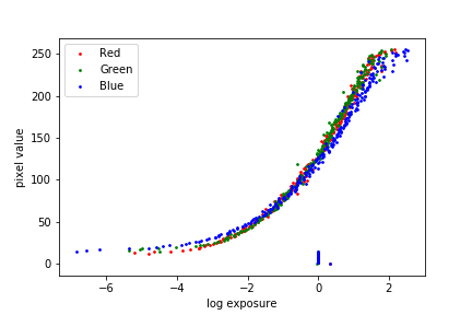 \(\lambda = 0\), identity weighting |
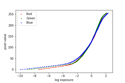 \(\lambda = 100\), identity weighting |
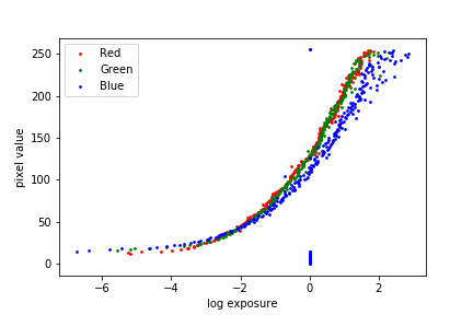 \(\lambda = 0\), tent weighting |
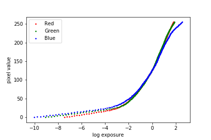 \(\lambda = 100\), tent weighting |
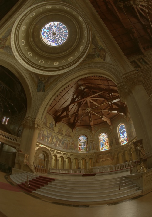
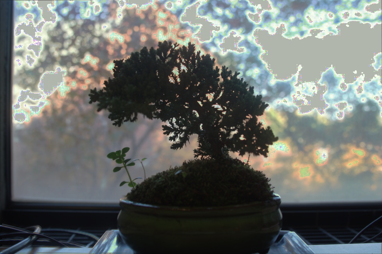
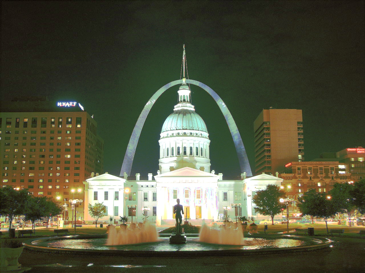
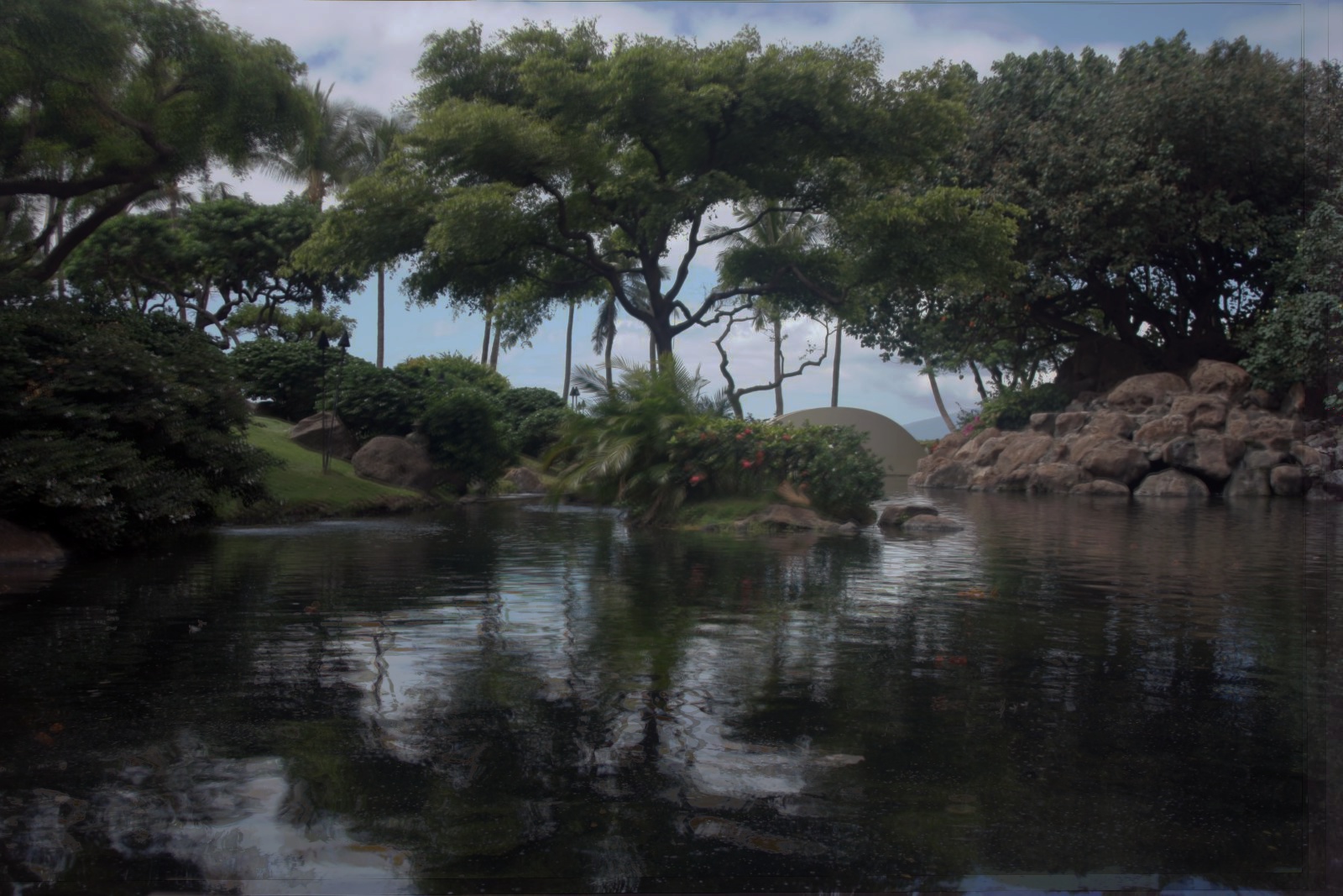
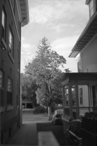
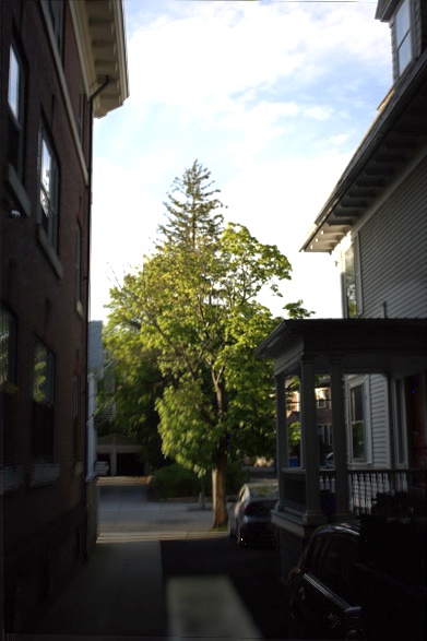
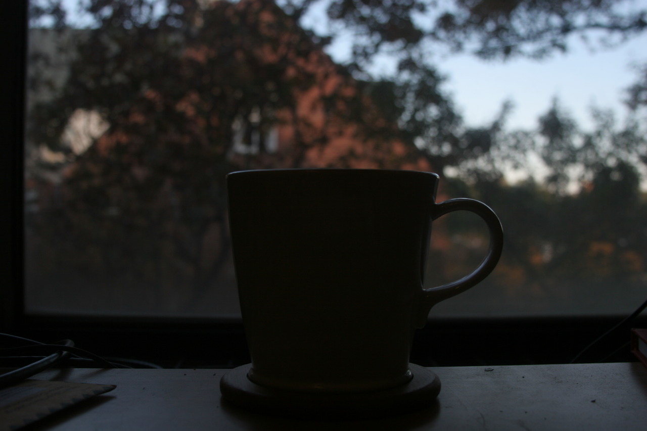
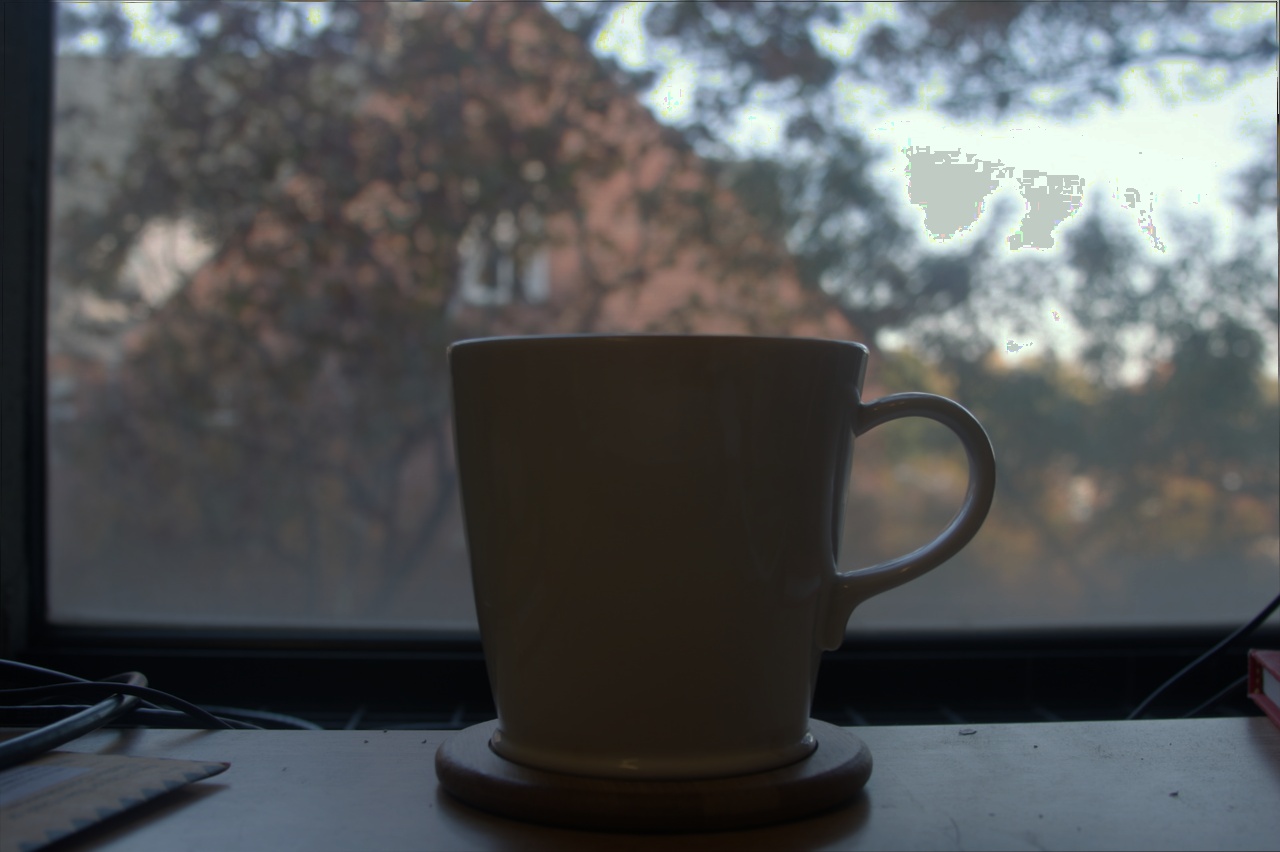
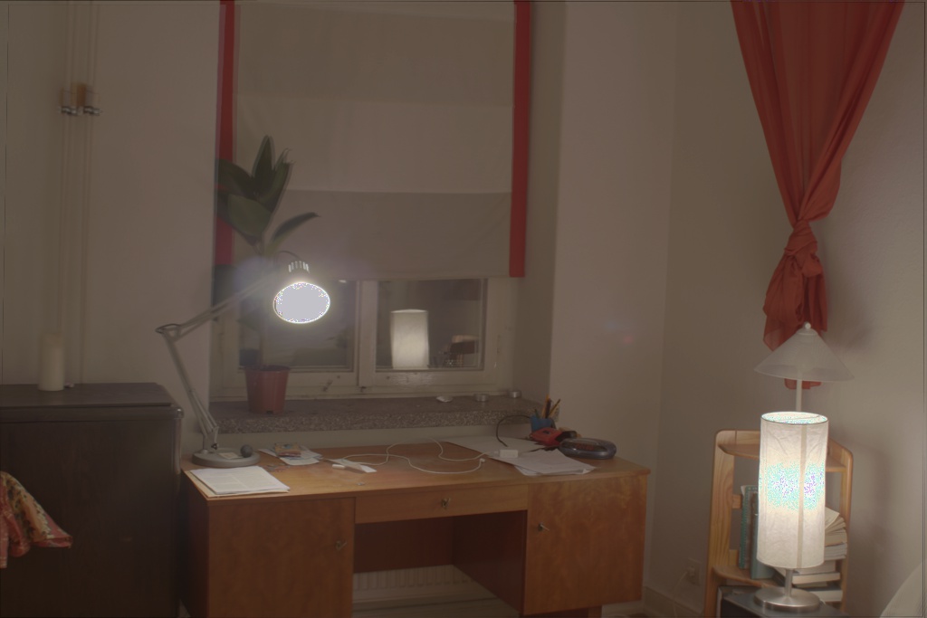
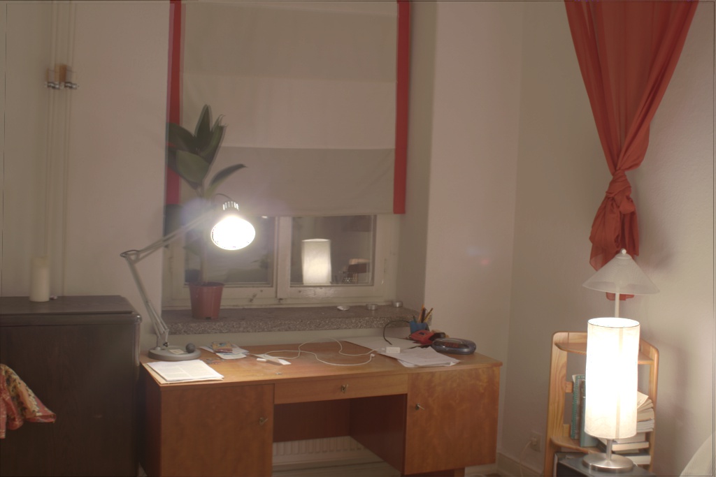
Obtaining the radiance map is only the first step of creaing a great HDR image. The next step is to show details in the dark and bright regions of the scene on a low-dynamic-range display. In this step, we implement both a global tone-mapping operator using gamma compression and a local tone-mapping operator following the paper by Fre ́do Durand and Julie Dorsey. The local tone-mapping algorithm is based on bilateral filtering, which decomposes the radiance map into high-frequency details and low-frequency structure.
The key insight of this local tone-mapping algorithm is that global tone-mapping operator often results in images that lack details, and one way to work around is separating out the large-scale variations and details. The algorithm starts by extracting the intensity of the original image \(I\) by taking the mean across three color channels. Then we apply bilateral filter to the intensity to get the large-scale variations image and the detail image. To preserve the details in the original image, instead of shrinking the dynamic range globally, we only reduce the contrast on the large-scale variation image. This results in an image that is both displayable on low-dynamic-range display and preserves the details.
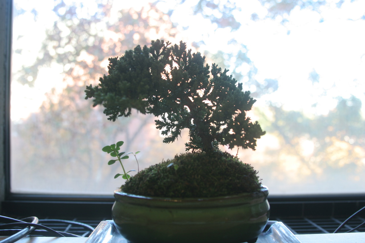
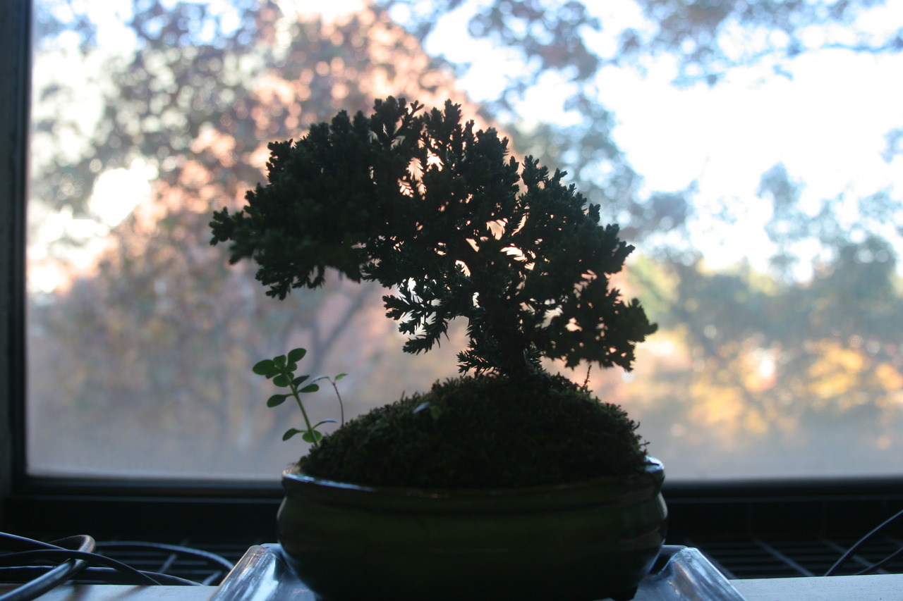
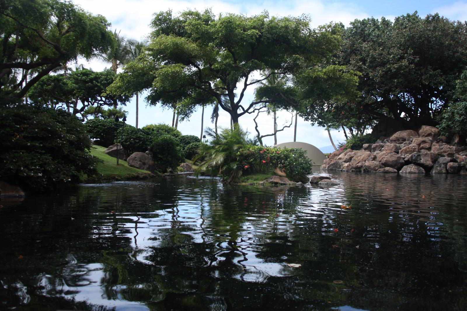
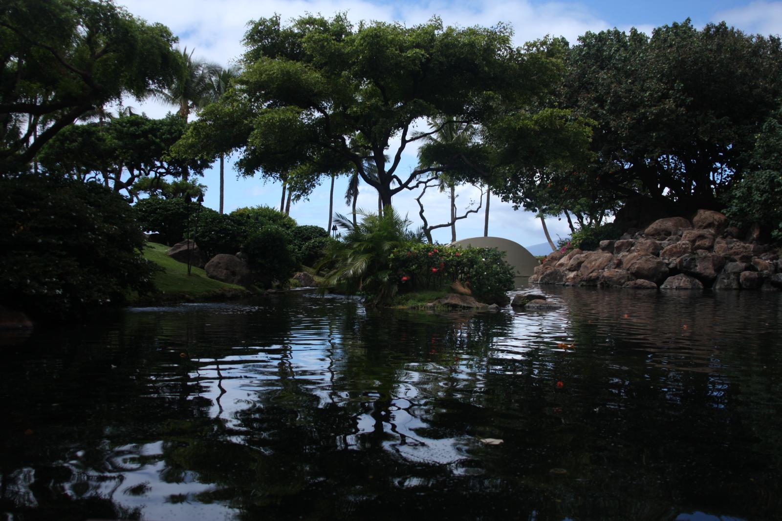
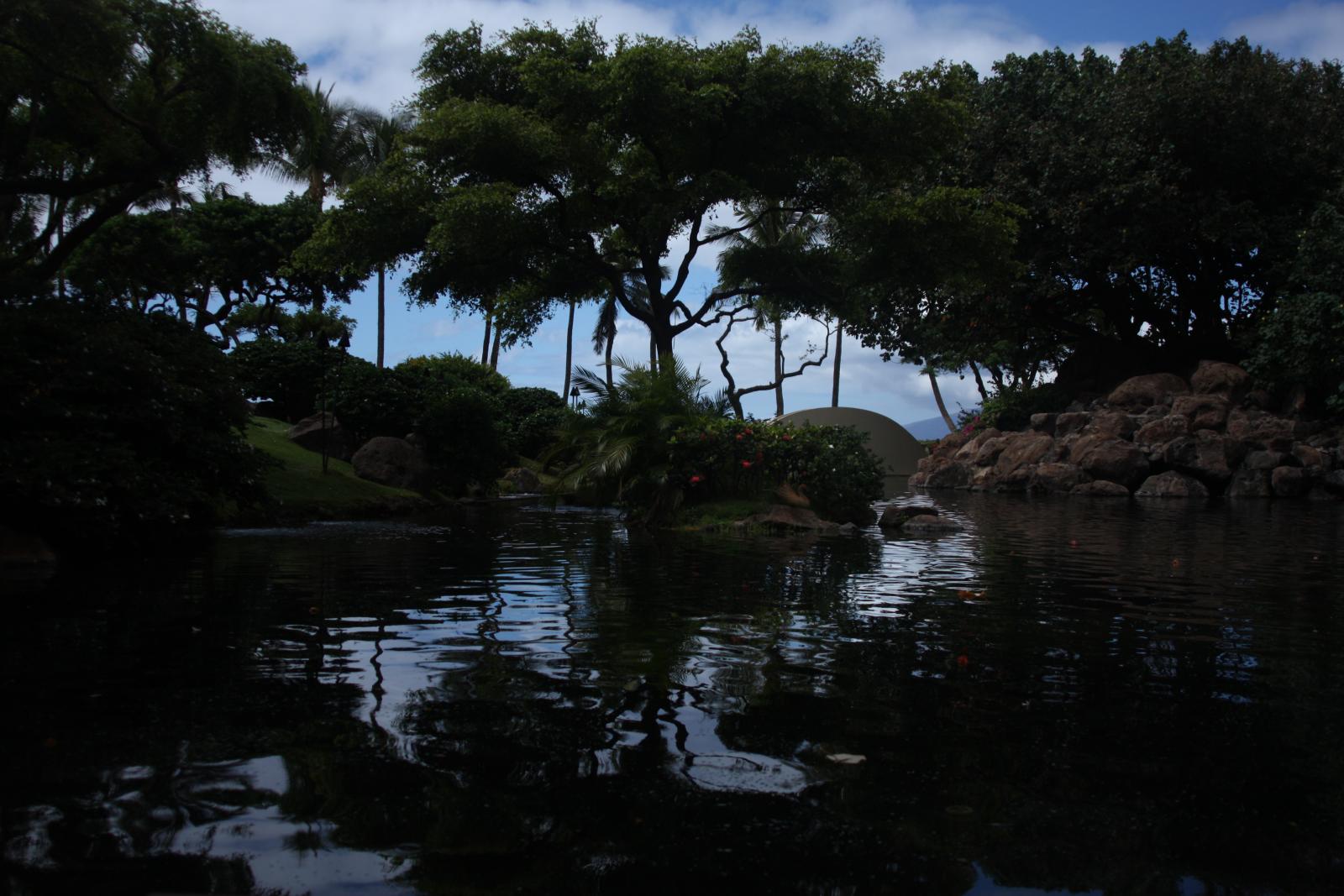
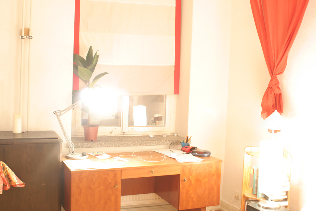
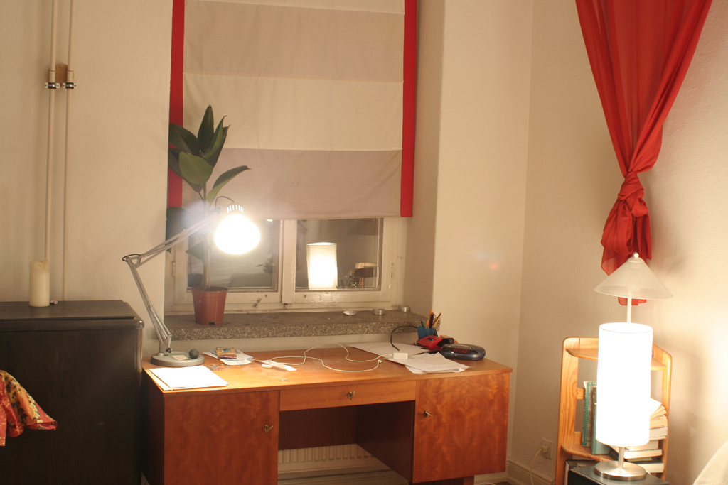
We show the final images obtained by both tone-mapping methods and the bilateral decomposition below.
Please zoom in to see the bilateral-filtered detail since the pixel values tend to have small variance and may not be visible at small scale.
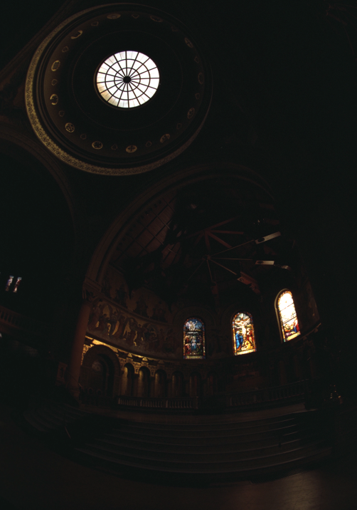
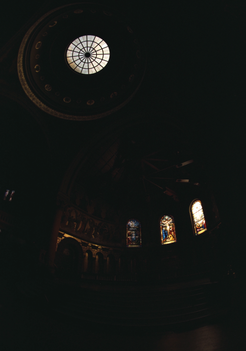
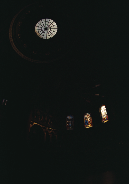
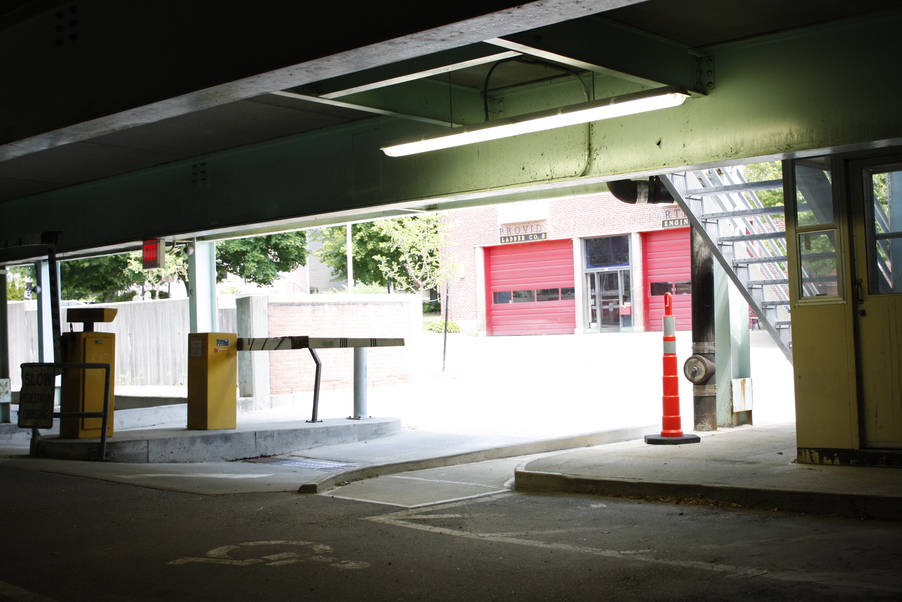
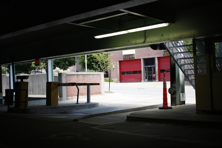
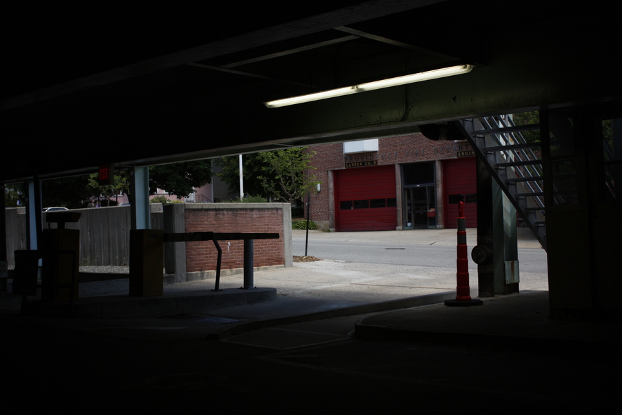
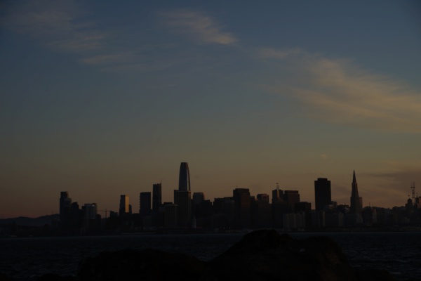
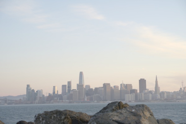
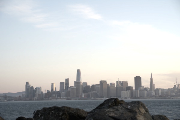
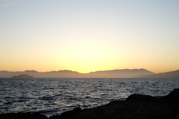
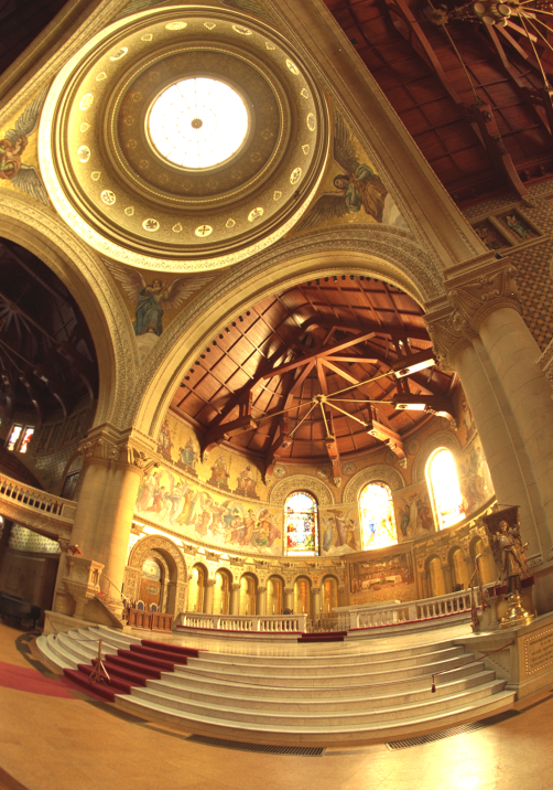 T = 8 seconds |
T = 4 seconds |
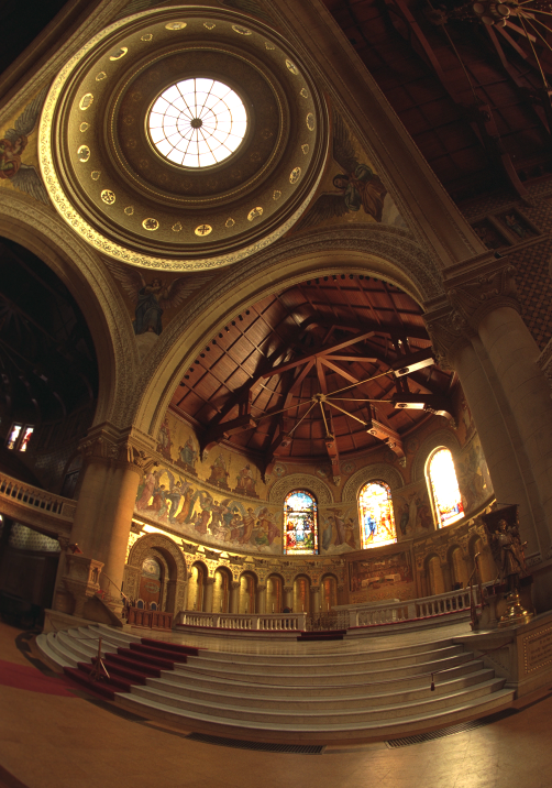 T = 2 seconds |
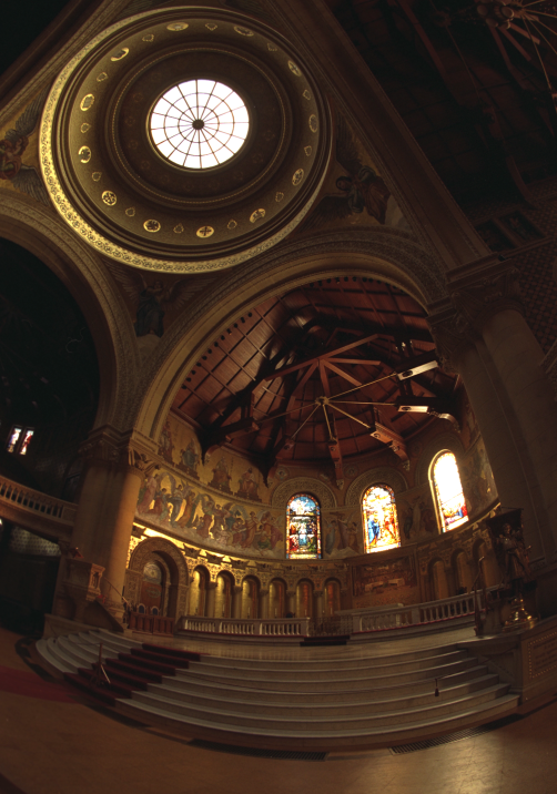 T = 1 second |
 T = 1/2 seconds |
 T = 1/4 seconds |
 T = 1/8 seconds |
 T = 1/16 second |
 T = 1/32 seconds |
 T = 1/64 seconds |
 T = 1/128 seconds |
 T = 1/256 second |
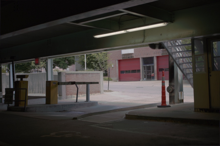
 Global Tone-Mapped HDR |
 Bilateral Filtered Detail |
 Bilateral Filtered Structure |
 Local Tone-Mapped HDR |
 T = 1/2 seconds |
 T = 1/4 seconds |
 T = 1/10 seconds |
 T = 1/25 seconds |
 Global Tone-Mapped HDR |
 Bilateral Filtered Detail |
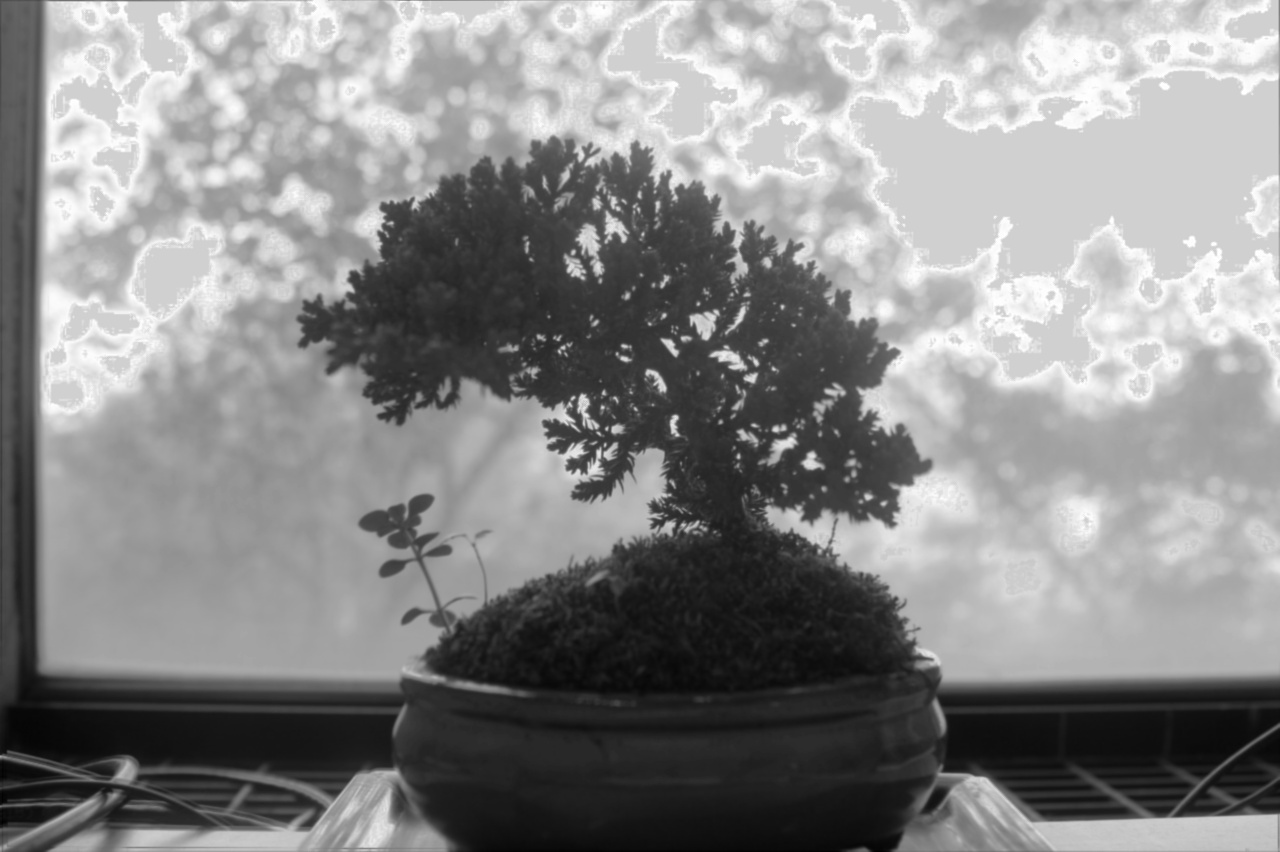 Bilateral Filtered Structure |
 Local Tone-Mapped HDR |
 T = 17 seconds |
 T = 3 seconds |
 T = 1/4 seconds |
 T = 1/25 seconds |
 Global Tone-Mapped HDR |
 Bilateral Filtered Detail |
 Bilateral Filtered Structure |
 Local Tone-Mapped HDR |
 T = 1/40 seconds |
 T = 1/160 seconds |
 T = 1/640 seconds |
 Global Tone-Mapped HDR |
 Bilateral Filtered Detail |
 Bilateral Filtered Structure |
 Local Tone-Mapped HDR |
 T = 1/160 seconds |
 T = 1/320 seconds |
 T = 1/800 seconds |
 T = 1/1600 seconds |
 T = 1/3200 seconds |
 Global Tone-Mapped HDR |
 Bilateral Filtered Detail |
 Bilateral Filtered Structure |
 Local Tone-Mapped HDR |
 T = 1/320 seconds |
T = 1/640 seconds |
 T = 1/1250 seconds |
 Global Tone-Mapped HDR |
 Bilateral Filtered Detail |
 Bilateral Filtered Structure |
 Local Tone-Mapped HDR |
 T = 1/8 seconds |
 T = 1/20 seconds |
 T = 1/40 seconds |
 T = 1/80 seconds |
 T = 1/160 seconds |
 Global Tone-Mapped HDR |
 Bilateral Filtered Detail |
 Bilateral Filtered Structure |
 Local Tone-Mapped HDR |
 T = 4 seconds |
 T = 1 second |
 T = 1/4 seconds |
 T = 1/15 seconds |
 T = 1/60 seconds |
 Global Tone-Mapped HDR |
 Bilateral Filtered Detail |
 Bilateral Filtered Structure |
 Local Tone-Mapped HDR |
 T = 1/5 seconds |
 T = 1/10 seconds |
 T = 1/15 seconds |
 T = 1/20 second |
 T = 1/40 seconds |
 T = 1/60 seconds |
 Global Tone-Mapped HDR |
 Local Tone-Mapped HDR |
 T = 1/30 seconds |
 T = 1/50 seconds |
 T = 1/60 seconds |
 T = 1/100 second |
 T = 1/160 seconds |
 T = 1/200 seconds |
 Global Tone-Mapped HDR |
 Local Tone-Mapped HDR |
Chapel image below. We can see that the image obtained with this method also achieves reasonable tone-mapping result, but it has high contrast and is not as bright as the the local tone-mapping method based on bilateral filter that we have shown above.
Bilateral Tone-Mapping |
 Template Tone-Mapping |
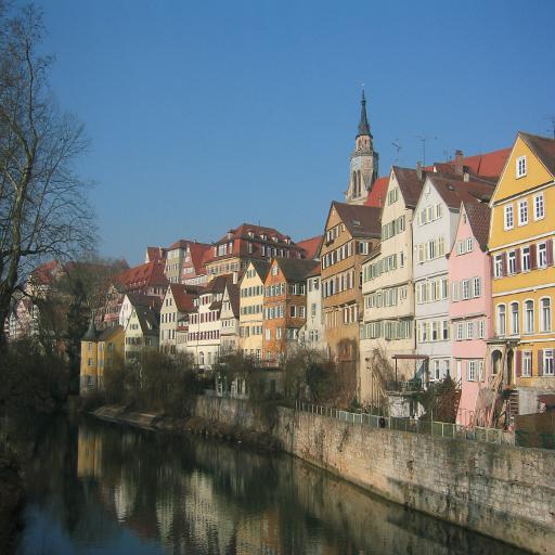
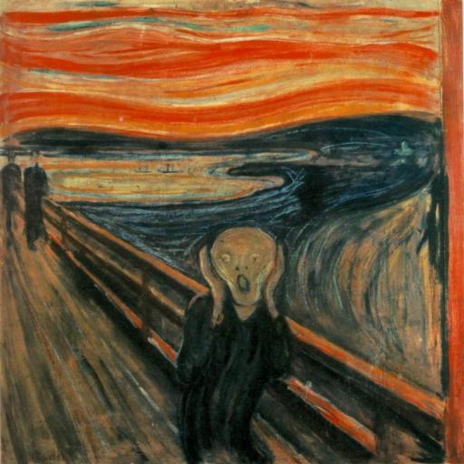
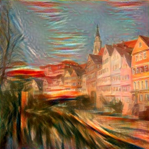
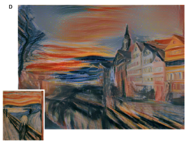
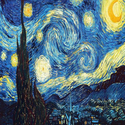
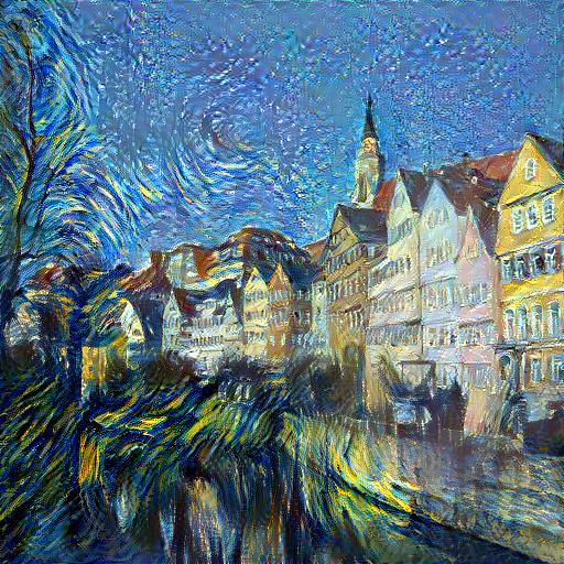
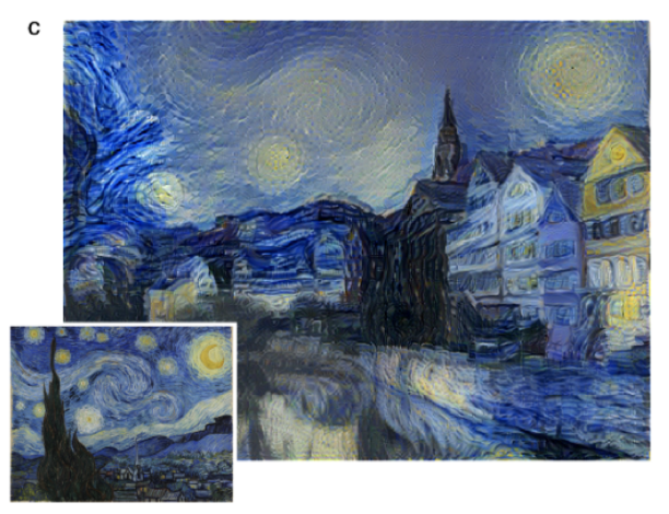
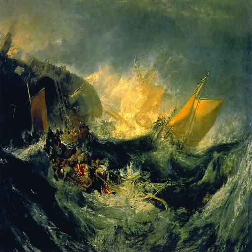
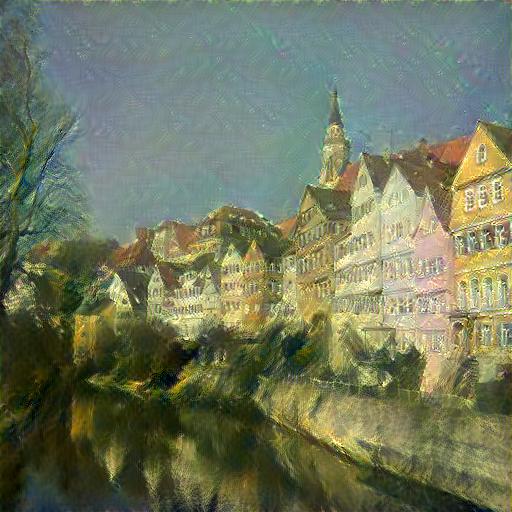
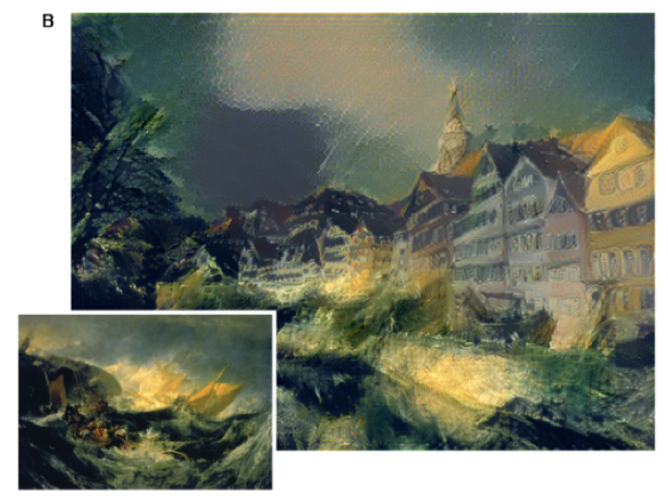
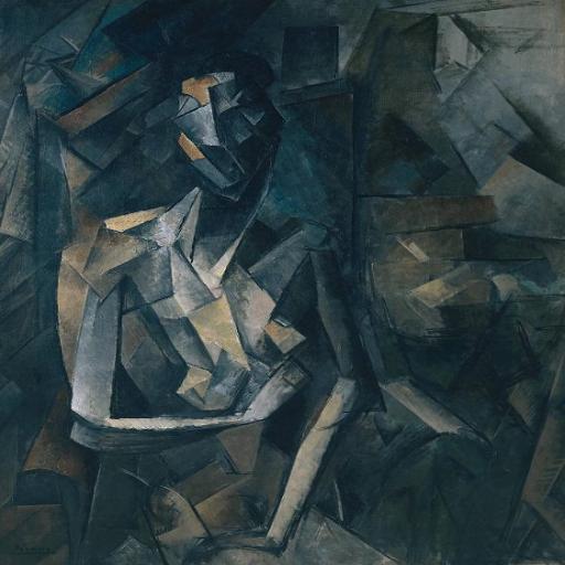
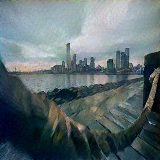
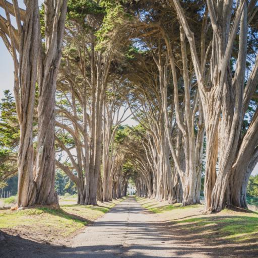
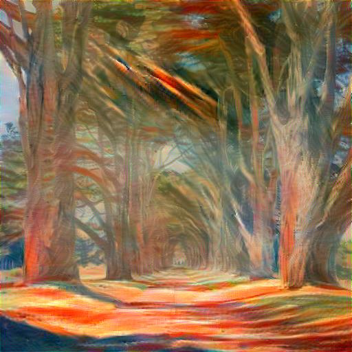
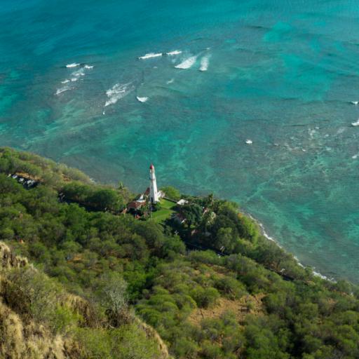
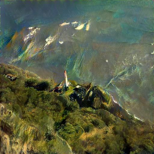
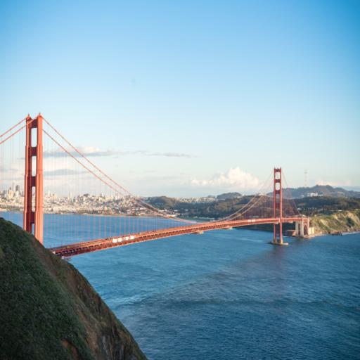
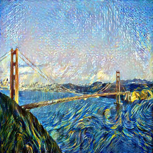
| Content Image | Style Image | Our Results | Paper Results |
 |
 |
 |
 |
|
 |
 |
 |
|
 |
 |
 |
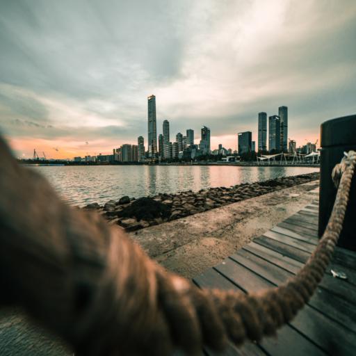
| Content Image | Style Image | Our Results |
 |
 |
 |
 |
|
 |
 |
|
 |
 |
|
 |
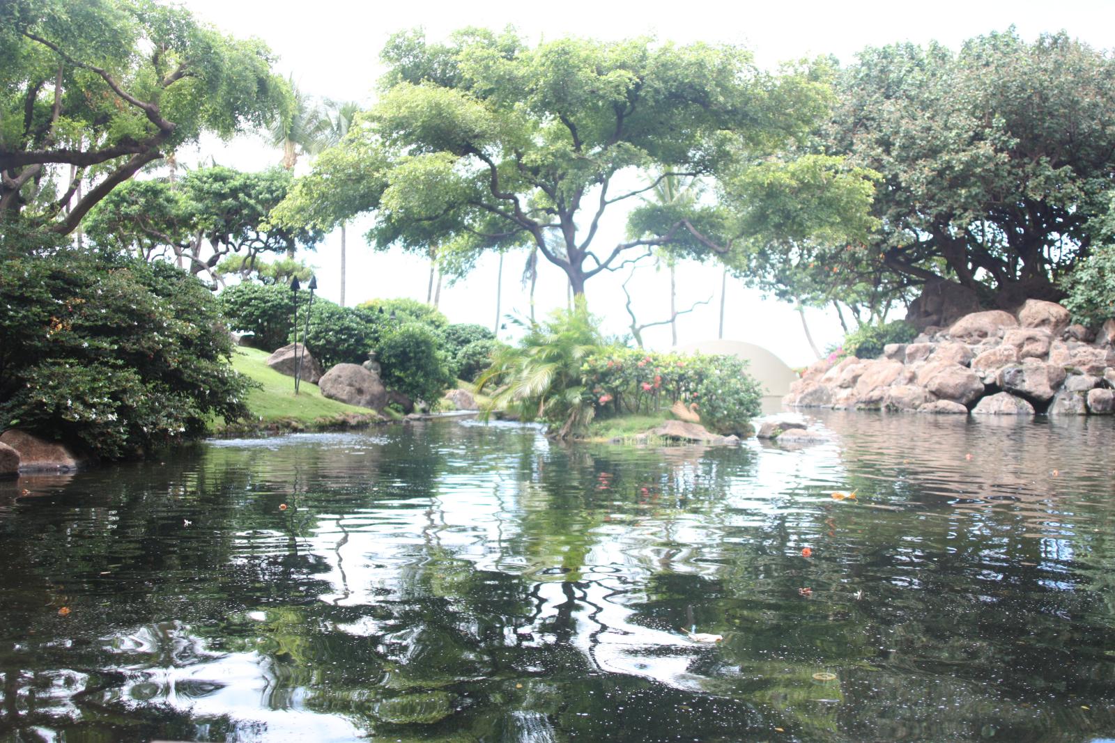
This project reproduces the lightfield effect proposed in this paper by Ng et al by using shifting and averaging operations on multiple images taken over a plane orthogonal to the optical axis. We use datasets each comprising of 289 images taken over a regularly spaced grid from the Stanford Light Field Archive.
The objects which are far away from the camera do not vary their position significantly when the camera moves around while keeping the optical axis direction unchanged. The nearby objects, on the other hand, vary their position significantly across images. Averaging all the images in the grid without any shifting will produce an image which is sharp around the far-away objects but blurry around the nearby ones, as shown by the following image:
 |
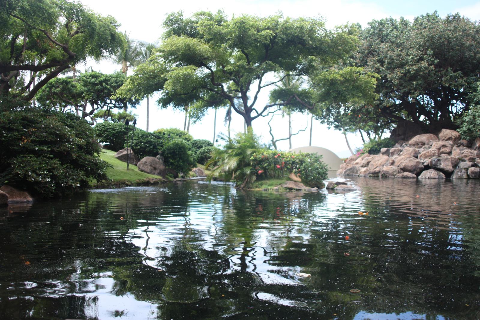
Shifting the images 'appropriately' and then averaging allows one to focus on object at different depths. To find out the 'appropriate' shift for each image, we extract the camera positions and grid indices from the image file names and build a 17x17 image grid using grid indices. Then we use the center image (with index [8, 8]) as the reference image, and calculate the distances from each image to the center image in both x and y axis. Multiplying the distances by a scalar factor scale gives the shifts that allow images refocused at different depths. A smaller scale results in a closer focus.
Below are the results with different shift scale factors, and the last gif shows the transition in different focus depth.
 scale = -0.27 |
 scale = -0.19 |
 scale = -0.11 |
 scale = -0.03 |
 |
 |
In this part we reproduce the aperture effect in lightfield photos by adjusting the number of images to be averaged. Averaging a large number of images sampled over the grid mimics a camera with a much larger aperture, while using fewer images simulates a smaller aperture. We define a radius parameter that represents the aperture and determines the images to be selected. We average images whose index is within radius away from the center image on the grid, that is, radius=0 means only select the center image and radius=8 means select all images on the grid. Below we show the image results with different apertures.
 radius = 2 |
 radius = 4 |
 radius = 6 |
 radius = 8 |
 |
 |
[1] Debevec, Paul E., and Jitendra Malik. "Recovering high dynamic range radiance maps from photographs." ACM SIGGRAPH 2008 classes. 2008. 1-10.
[2] Durand, Frédo, and Julie Dorsey. "Fast bilateral filtering for the display of high-dynamic-range images." Proceedings of the 29th annual conference on Computer graphics and interactive techniques. 2002.
[3] HDR Dataset from the HDR assignment from the Computational Photography course at Brown University.
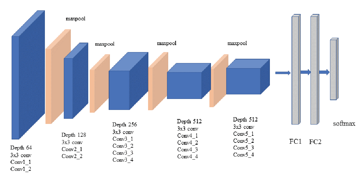
[4] Gatys, Leon A., Alexander S. Ecker, and Matthias Bethge. "A neural algorithm of artistic style." arXiv preprint arXiv:1508.06576 (2015).
[5] Ng, Ren, et al. "Light field photography with a hand-held plenoptic camera." Computer Science Technical Report CSTR 2.11 (2005): 1-11.