2.2.1   Example: Arithmetic on Rational Numbers

Recall that a rational number is a ratio of integers, and rational numbers constitute an important sub-class of real numbers. A rational number like 1/3 or 17/29 is typically written as:

<numerator>/<denominator>

where both the <numerator> and <denominator> are placeholders for integer values. Both parts are needed to exactly characterize the value of the rational number.

Rational numbers are important in computer science because they, like integers, can be represented exactly. Irrational numbers (like \(\pi\) or \(e\) or \(\sqrt{2}\)) are instead approximated using a finite binary expansion. Thus, working with rational numbers should, in principle, allow us to avoid approximation errors in our arithmetic.

However, as soon as we actually divide the numerator by the denominator, we can be left with a truncated decimal approximation (a float):

>>> 1/3
0.3333333333333333

and the problems with this approximation appear when we start to conduct tests:

>>> 1/3 == 0.333333333333333300000  # Beware of approximations
True

How computers approximate real numbers with finite-length decimal expansions is a topic for another class. The important idea here is that by representing rational numbers as ratios of integers, we avoid the approximation problem entirely. Hence, we would like to keep the numerator and denominator separate for the sake of precision, but treat them as a single unit.

We know from using functional abstractions that we can start programming productively before we have an implementation of some parts of our program. Let us begin by assuming that we already have a way of constructing a rational number from a numerator and a denominator, available as a constructor. We also assume that, given a rational number, we have ways of extracting (or selecting) its numerator and its denominator, available as selectors. The constructor and selectors can be the following three functions:

• make_rat(n, d) returns the rational number with numerator n and denominator d.
• numer(x) returns the numerator of the rational number x.
• denom(x) returns the denominator of the rational number x.

We are using here a powerful strategy of synthesis: wishful thinking. We haven't yet said how a rational number is represented, or how the functions numer, denom, and make_rat should be implemented. Even so, if we did have these three functions, we could then add, multiply, and test equality of rational numbers by calling them:

>>> def add_rat(x, y):
        nx, dx = numer(x), denom(x)
        ny, dy = numer(y), denom(y)
        return make_rat(nx * dy + ny * dx, dx * dy)

>>> def mul_rat(x, y):
        return make_rat(numer(x) * numer(y), denom(x) * denom(y))

>>> def eq_rat(x, y):
        return numer(x) * denom(y) == numer(y) * denom(x)

Now we have the operations on rational numbers defined in terms of the selector functions numer and denom, and the constructor function make_rat, but we haven't yet defined these functions. What we need is some way to glue together a numerator and a denominator into a unit.

2.2.2   Tuples

To enable us to implement the concrete level of our data abstraction, Python provides a compound structure called a tuple, which can be constructed by separating values by commas. Although not strictly required, parentheses almost always surround tuples.

>>> (1, 2)
(1, 2)

The elements of a tuple can be unpacked in two ways. The first way is via our familiar method of multiple assignment.

>>> pair = (1, 2)
>>> pair
(1, 2)
>>> x, y = pair
>>> x
1
>>> y
2

In fact, multiple assignment has been creating and unpacking tuples all along.

A second method for accessing the elements in a tuple is by the indexing operator, written as square brackets.

>>> pair[0]
1
>>> pair[1]
2

Tuples in Python (and sequences in most other programming languages) are 0-indexed, meaning that the index 0 picks out the first element, index 1 picks out the second, and so on. One intuition that underlies this indexing convention is that the index represents how far an element is offset from the beginning of the tuple.

The equivalent function for the element selection operator is called getitem, and it also uses 0-indexed positions to select elements from a tuple.

>>> from operator import getitem
>>> getitem(pair, 0)
1

Tuples are native types, which means that there are built-in Python operators to manipulate them. We'll return to the full properties of tuples shortly. At present, we are only interested in how tuples can serve as the glue that implements abstract data types.

Representing Rational Numbers. Tuples offer a natural way to implement rational numbers as a pair of two integers: a numerator and a denominator. We can implement our constructor and selector functions for rational numbers by manipulating 2-element tuples.

>>> def make_rat(n, d):
        return (n, d)

>>> def numer(x):
        return getitem(x, 0)

>>> def denom(x):
        return getitem(x, 1)

A function for printing rational numbers completes our implementation of this abstract data type.

>>> def str_rat(x):
        """Return a string 'n/d' for numerator n and denominator d."""
        return '{0}/{1}'.format(numer(x), denom(x))

Together with the arithmetic operations we defined earlier, we can manipulate rational numbers with the functions we have defined.

>>> half = make_rat(1, 2)
>>> str_rat(half)
'1/2'
>>> third = make_rat(1, 3)
>>> str_rat(mul_rat(half, third))
'1/6'
>>> str_rat(add_rat(third, third))
'6/9'

As the final example shows, our rational-number implementation does not reduce rational numbers to lowest terms. We can remedy this by changing make_rat. If we have a function for computing the greatest common denominator of two integers, we can use it to reduce the numerator and the denominator to lowest terms before constructing the pair. As with many useful tools, such a function already exists in the Python Library.

>>> from fractions import gcd
>>> def make_rat(n, d):
        g = gcd(n, d)
        return (n//g, d//g)

The double slash operator, //, expresses integer division, which rounds down the fractional part of the result of division. Since we know that g divides both n and d evenly, integer division is exact in this case. Now we have

>>> str_rat(add_rat(third, third))
'2/3'

as desired. This modification was accomplished by changing the constructor without changing any of the functions that implement the actual arithmetic operations.

Further reading. The str_rat implementation above uses format strings, which contain placeholders for values. The details of how to use format strings and the format method appear in the formatting strings section of Dive Into Python 3.

2.2.3   Abstraction Barriers

Before continuing with more examples of compound data and data abstraction, let us consider some of the issues raised by the rational number example. We defined operations in terms of a constructor make_rat and selectors numer and denom. In general, the underlying idea of data abstraction is to identify for each type of value a basic set of operations in terms of which all manipulations of values of that type will be expressed, and then to use only those operations in manipulating the data.

We can envision the structure of the rational number system as a series of layers.

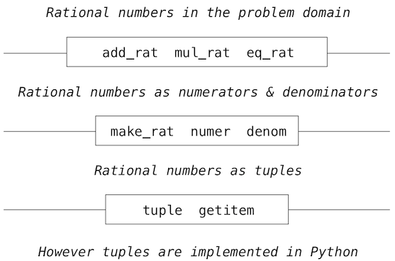
The horizontal lines represent abstraction barriers that isolate different levels of the system. At each level, the barrier separates the functions (above) that use the data abstraction from the functions (below) that implement the data abstraction. Programs that use rational numbers manipulate them solely in terms of the their arithmetic functions: add_rat, mul_rat, and eq_rat. These, in turn, are implemented solely in terms of the constructor and selectors make_rat, numer, and denom, which themselves are implemented in terms of tuples. The details of how tuples are implemented are irrelevant to the rest of the layers as long as tuples enable the implementation of the selectors and constructor.

At each layer, the functions within the box enforce the abstraction boundary because they are the only functions that depend upon both the representation above them (by their use) and the implementation below them (by their definitions). In this way, abstraction barriers are expressed as sets of functions.

Abstraction barriers provide many advantages. One advantage is that they makes programs much easier to maintain and to modify. The fewer functions that depend on a particular representation, the fewer changes are required when one wants to change that representation.

2.2.4   The Properties of Data

We began the rational-number implementation by implementing arithmetic operations in terms of three unspecified functions: make_rat, numer, and denom. At that point, we could think of the operations as being defined in terms of data objects --- numerators, denominators, and rational numbers --- whose behavior was specified by the latter three functions.

But what exactly is meant by data? It is not enough to say "whatever is implemented by the given selectors and constructors." We need to guarantee that these functions together specify the right behavior. That is, if we construct a rational number x from integers n and d, then it should be the case that numer(x)/denom(x) is equal to n/d.

In general, we can think of an abstract data type as defined by some collection of selectors and constructors, together with some behavior conditions. As long as the behavior conditions are met (such as the division property above), these functions constitute a valid representation of the data type.

This point of view can be applied to other data types as well, such as the two-element tuple that we used in order to implement rational numbers. We never actually said much about what a tuple was, only that the language supplied operators to create and manipulate tuples. We can now describe the behavior conditions of two-element tuples, also called pairs, that are relevant to the problem of representing rational numbers.

To implement rational numbers, we needed a glue for two integers, which had the following behavior:

• If a pair p was constructed from values x and y, then getitem_pair(p, 0) returns x, and getitem_pair(p, 1) returns y.

We can implement functions make_pair and getitem_pair that fulfill this description just as well as a tuple.

>>> def make_pair(x, y):
        """Return a function that behaves like a pair."""
        def dispatch(m):
            if m == 0:
                return x
            elif m == 1:
                return y
        return dispatch

>>> def getitem_pair(p, i):
        """Return the element at index i of pair p."""
        return p(i)

With this implementation, we can create and manipulate pairs.

>>> p = make_pair(1, 2)
>>> getitem_pair(p, 0)
1
>>> getitem_pair(p, 1)
2

This use of functions corresponds to nothing like our intuitive notion of what data should be. Nevertheless, these functions suffice to represent compound data in our programs.

The subtle point to notice is that the value returned by make_pair is a function called dispatch, which takes an argument m and returns either x or y. Then, getitem_pair calls this function to retrieve the appropriate value. We will return to the topic of dispatch functions in the next chapter.

The point of exhibiting the functional representation of a pair is not that Python actually works this way (tuples are implemented more directly, for efficiency reasons) but that it could work this way. The functional representation, although obscure, is a perfectly adequate way to represent pairs, since it fulfills the only conditions that pairs need to fulfill. This example also demonstrates that the ability to manipulate functions as values automatically provides us the ability to represent compound data.

2.3.1   Tuples Again

The tuple type that we were introduced to is itself a full sequence type. Tuples provide substantially more functionality than the pair abstract data type that we implemented functionally.

Tuples can have arbitrary length, and they exhibit the two principal behaviors of the sequence abstraction: length and element selection. Below, digits is a tuple with four elements.

>>> digits = (1, 8, 2, 8)
>>> len(digits)
4
>>> digits[3]
8

Additionally, tuples can be added together and multiplied by integers. For tuples, addition and multiplication do not add or multiply elements, but instead combine and replicate the tuples themselves. That is, the add function in the operator module (and the + operator) returns a new tuple that is the concatenation of the added arguments. The mul function in operator (and the * operator) can take an integer k and a tuple and return a new tuple that consists of k copies of the tuple argument.

>>> (2, 7) + digits * 2
(2, 7, 1, 8, 2, 8, 1, 8, 2, 8)

Mapping. A powerful method of transforming one tuple into another is by applying a function to each element and collecting the results. This general form of computation is called mapping a function over a sequence, and corresponds to the built-in function map. The result of map is an object that is not itself a sequence, but can be converted into a sequence by calling tuple, the constructor function for tuples.

>>> alternates = (-1, 2, -3, 4, -5)
>>> tuple(map(abs, alternates))
(1, 2, 3, 4, 5)

The map function is important because it relies on the sequence abstraction: we do not need to be concerned about the structure of the underlying tuple; only that we can access each one of its elements individually in order to pass it as an argument to the mapped function (abs, in this case).

2.3.2   Sequence Iteration

Mapping is itself an instance of a general pattern of computation: iterating over all elements in a sequence. To map a function over a sequence, we do not just select a particular element, but each element in turn. This pattern is so common that Python has an additional control statement to process sequential data: the for statement.

Consider the problem of counting how many times a value appears in a sequence. We can implement a function to compute this count using a while loop.

>>> def count(s, value):
        """Count the number of occurrences of value in sequence s."""
        total, index = 0, 0
        while index < len(s):
            if s[index] == value:
                total = total + 1
            index = index + 1
        return total

>>> count(digits, 8)
2

The Python for statement can simplify this function body by iterating over the element values directly, without introducing the name index at all. For example (pun intended), we can write:

>>> def count(s, value):
        """Count the number of occurrences of value in sequence s."""
        total = 0
        for elem in s:
            if elem == value:
                total = total + 1
        return total

>>> count(digits, 8)
2

A for statement consists of a single clause with the form:

for <name> in <expression>:
    <suite>

A for statement is executed by the following procedure:

1. Evaluate the header <expression>, which must yield an iterable value.
2. For each element value in that sequence, in order:
   1. Bind <name> to that value in the local environment.
   2. Execute the <suite>.

Step 1 refers to an iterable value. Sequences are iterable, and their elements are considered in their sequential order. Python does include other iterable types, but we will focus on sequences for now; the general definition of the term "iterable" appears in the section on iterators in Chapter 4.

An important consequence of this evaluation procedure is that <name> will be bound to the last element of the sequence after the for statement is executed. The for loop introduces yet another way in which the local environment can be updated by a statement.

Sequence unpacking. A common pattern in programs is to have a sequence of elements that are themselves sequences, but all of a fixed length. For statements may include multiple names in their header to "unpack" each element sequence into its respective elements. For example, we may have a sequence of pairs (that is, two-element tuples),

>>> pairs = ((1, 2), (2, 2), (2, 3), (4, 4))

and wish to find the number of pairs that have the same first and second element.

>>> same_count = 0

The following for statement with two names in its header will bind each name x and y to the first and second elements in each pair, respectively.

>>> for x, y in pairs:
        if x == y:
            same_count = same_count + 1

>>> same_count
2

This pattern of binding multiple names to multiple values in a fixed-length sequence is called sequence unpacking; it is the same pattern that we see in assignment statements that bind multiple names to multiple values.

Ranges. A range is another built-in type of sequence in Python, which represents a range of integers. Ranges are created with the range function, which takes two integer arguments: the first number and one beyond the last number in the desired range.

>>> range(1, 10)  # Includes 1, but not 10
range(1, 10)

Calling the tuple constructor on a range will create a tuple with the same elements as the range, so that the elements can be easily inspected.

>>> tuple(range(5, 8))
(5, 6, 7)

If only one argument is given, it is interpreted as one beyond the last value for a range that starts at 0.

>>> tuple(range(4))
(0, 1, 2, 3)

Ranges commonly appear as the expression in a for header to specify the number of times that the suite should be executed:

>>> total = 0
>>> for k in range(5, 8):
        total = total + k

>>> total
18

A common convention is to use a single underscore character for the name in the for header if the name is unused in the suite:

>>> for _ in range(3):
        print('Go Bears!')

Go Bears!
Go Bears!
Go Bears!

Note that an underscore is just another name in the environment as far as the interpreter is concerned, but has a conventional meaning among programmers that indicates the name will not appear in any expressions.

2.3.3   Sequence Abstraction

We have now introduced two types of native data types that implement the sequence abstraction: tuples and ranges. Both satisfy the conditions with which we began this section: length and element selection. Python includes two more behaviors of sequence types that extend the sequence abstraction.

Membership. A value can be tested for membership in a sequence. Python has two operators in and not in that evaluate to True or False depending on whether an element appears in a sequence.

>>> digits
(1, 8, 2, 8)
>>> 2 in digits
True
>>> 1828 not in digits
True

All sequences also have methods called index, which return the index of a value in a sequence, and count, which returns the count of a value in a sequence.

>>> digits.index(2)
2
>>> digits.count(8)
2

Slicing. Sequences contain smaller sequences within them. We observed this property when developing our nested pairs implementation, which decomposed a sequence into its first element and the rest. A slice of a sequence is any span of the original sequence, designated by a pair of integers. As with the range constructor, the first integer indicates the starting index of the slice and the second indicates one beyond the ending index.

In Python, sequence slicing is expressed similarly to element selection, using square brackets. A colon separates the starting and ending indices. Any bound that is omitted is assumed to be an extreme value: 0 for the starting index, and the length of the sequence for the ending index.

>>> digits[0:2]
(1, 8)
>>> digits[1:]
(8, 2, 8)
>>> digits[:3]
(1, 8, 2)

Enumerating these additional behaviors of the Python sequence abstraction gives us an opportunity to reflect upon what constitutes a useful data abstraction in general. The richness of an abstraction (that is, how many behaviors it includes) has consequences. For users of an abstraction, additional behaviors can be helpful. On the other hand, satisfying the requirements of a rich abstraction with a new data type can be challenging. To ensure that our implementations of pther abstract data types support these additional behaviors would require some work. Another negative consequence of rich abstractions is that they take longer for users to learn.

Sequences have a rich abstraction because they are so ubiquitous in computing that learning a few complex behaviors is justified. In general, most user-defined abstractions should be kept as simple as possible.

Further reading. Slice notation admits a variety of special cases, such as negative starting values, ending values, and step sizes. A complete description appears in the subsection called slicing a list in Dive Into Python 3. In this chapter, we will only use the basic features described above.

2.3.4   Strings

Text values are perhaps more fundamental to computer science than even numbers. As a case in point, Python programs are written and stored as text. The native data type for text in Python is called a string, and corresponds to the constructor str.

There are many details of how strings are represented, expressed, and manipulated in Python. Strings are another example of a rich abstraction, one which requires a substantial commitment on the part of the programmer to master. This section serves as a condensed introduction to essential string behaviors.

String literals can express arbitrary text, surrounded by either single or double quotation marks. However, the string must be surrounded by the same kind of quotation marks: if you start the string with a single quotation mark, you must end it with a single quotation work. This allows us to have apostrophes within strings, as shown below.

>>> 'I am a string!'
'I am a string!'
>>> "I've got an apostrophe"
"I've got an apostrophe"
>>> '您好'
'您好'

We have seen strings already in our code, as docstrings, in calls to print, and as error messages in assert statements.

Strings satisfy the two basic conditions of a sequence that we introduced at the beginning of this section: they have a length and they support element selection.

>>> city = 'Berkeley'
>>> len(city)
8
>>> city[3]
'k'

The elements of a string are themselves strings that have only a single character. A character is any single letter of the alphabet, punctuation mark, or other symbol. Unlike many other programming languages, Python does not have a separate character type; any text is a string, and strings that represent single characters have a length of 1.

Like tuples, strings can also be combined via addition and multiplication.

>>> 'Berkeley' + ', CA'
'Berkeley, CA'
>>> 'Shabu ' * 2
'Shabu Shabu '

Membership. The behavior of strings diverges from other sequence types in Python. The string abstraction does not conform to the full sequence abstraction that we described for tuples and ranges. In particular, the membership operator in applies to strings, but has an entirely different behavior than when it is applied to sequences. It matches substrings rather than elements.

>>> 'here' in "Where's Waldo?"
True

Likewise, the count and index methods on strings take substrings as arguments, rather than single-character elements. The behavior of count is particularly nuanced; it counts the number of non-overlapping occurrences of a substring in a string.

>>> 'Mississippi'.count('i')
4
>>> 'Mississippi'.count('issi')
1

Multiline Literals. Strings aren't limited to a single line. Triple quotes delimit string literals that span multiple lines. We have used this triple quoting extensively already for docstrings.

>>> """The Zen of Python
claims, Readability counts.
Read more: import this."""
'The Zen of Python\nclaims, "Readability counts."\nRead more: import this.'

In the printed result above, the \n (pronounced "backslash en") is a single element that represents a new line. Although it appears as two characters (backslash and "n"), it is considered a single character for the purposes of length and element selection.

String Coercion. A string can be created from any object in Python by calling the str constructor function with an object value as its argument. This feature of strings is useful for constructing descriptive strings from objects of various types.

>>> str(2) + ' is an element of ' + str(digits)
'2 is an element of (1, 8, 2, 8)'

The mechanism by which a single str function can apply to any type of argument and return an appropriate value is the subject of the later section on generic functions.

Methods. The behavior of strings in Python is extremely productive because of a rich set of methods for returning string variants and searching for contents. A few of these methods are introduced below by example.

>>> '1234'.isnumeric()
True
>>> 'rOBERT dE nIRO'.swapcase()
'Robert De Niro'
>>> 'snakeyes'.upper().endswith('YES')
True

Further reading. Encoding text in computers is a complex topic. In this chapter, we will abstract away the details of how strings are represented. However, for many applications, the particular details of how strings are encoded by computers is essential knowledge. Sections 4.1-4.3 of Dive Into Python 3 provides a description of character encodings and Unicode.

2.3.5   Conventional Interfaces

In working with compound data, we've stressed how data abstraction permits us to design programs without becoming enmeshed in the details of data representations, and how abstraction preserves for us the flexibility to experiment with alternative representations. In this section, we introduce another powerful design principle for working with data structures --- the use of conventional interfaces.

A conventional interface is a data format that is shared across many modular components, which can be mixed and matched to perform data processing. For example, if we have several functions that all take a sequence as an argument and return a sequence as a value, then we can apply each to the output of the next in any order we choose. In this way, we can create a complex process by chaining together a pipeline of functions, each of which is simple and focused.

This section has a dual purpose: to introduce the idea of organizing a program around a conventional interface, and to demonstrate examples of modular sequence processing.

Consider these two problems, which appear at first to be related only in their use of sequences:

1. Sum the even members of the first n Fibonacci numbers.
2. List the letters in the acronym for a name, which includes the first letter of each capitalized word.

These problems are related because they can be decomposed into simple operations that take sequences as input and yield sequences as output. Moreover, those operations are instances of general methods of computation over sequences. Let's consider the first problem. It can be decomposed into the following steps, reading from left to right, where the output of one step is the input to the next step:

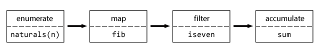
The fib function below computes Fibonacci numbers, now updated from the definition in Chapter 1 with a for statement and a range:

>>> def fib(k):
        """Compute the kth Fibonacci number."""
        prev, curr = 1, 0  # curr is the first Fibonacci number.
        for _ in range(k - 1):
             prev, curr = curr, prev + curr
        return curr

and a predicate iseven can be defined using the integer remainder operator, %.

>>> def iseven(n):
        return n % 2 == 0

The functions map and filter are operations on sequences. We have already encountered map, which applies a function to each element in a sequence and collects the results. The filter function takes a sequence and returns those elements of a sequence for which a predicate is true. Both of these functions return intermediate objects, map and filter objects, which are iterable objects that can be converted into tuples or summed.

>>> nums = (5, 6, -7, -8, 9)
>>> tuple(filter(iseven, nums))
(6, -8)
>>> sum(map(abs, nums))
35

Now we can implement even_fib, the solution to our first problem, in terms of map, filter, and sum.

>>> def sum_even_fibs(n):
        """Sum the first n even Fibonacci numbers."""
        return sum(filter(iseven, map(fib, range(1, n+1))))

>>> sum_even_fibs(20)
3382

Now, let's consider the second problem. It can also be decomposed as a pipeline of sequence operations that include map and filter:

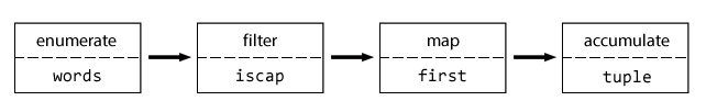
The words in a string can be enumerated via the split method of a string object, which by default splits on spaces.

>>> tuple('Spaces between words'.split())
('Spaces', 'between', 'words')

The first letter of a word can be retrieved using the selection operator, and a predicate that determines if a word is capitalized can be defined using the built-in predicate isupper.

>>> def first(s):
        return s[0]

>>> def iscap(s):
        return len(s) > 0 and s[0].isupper()

At this point, our acronym function can be defined via map and filter.

>>> def acronym(name):
        """Return a tuple of the letters that form the acronym for name."""
        return tuple(map(first, filter(iscap, name.split())))

>>> acronym('University of California Berkeley Undergraduate Graphics Group')
('U', 'C', 'B', 'U', 'G', 'G')

These similar solutions to rather different problems show how to combine general components that operate on the conventional interface of a sequence using the general computational patterns of mapping, filtering, and accumulation. The sequence abstraction allows us to specify these solutions concisely.

Expressing programs as sequence operations helps us design programs that are modular. That is, our designs are constructed by combining relatively independent pieces, each of which transforms a sequence. In general, we can encourage modular design by providing a library of standard components together with a conventional interface for connecting the components in flexible ways.

Generator expressions. The Python language includes a second approach to processing sequences, called generator expressions, which provide similar functionality to map and filter, but may require fewer function definitions.

Generator expressions combine the ideas of filtering and mapping together into a single expression type with the following form:

<map expression> for <name> in <sequence expression> if <filter expression>

To evaluate a generator expression, Python evaluates the <sequence expression>, which must return an iterable value. Then, for each element in order, the element value is bound to <name>, the <filter expression> is evaluated, and if it yields a true value, the <map expression> is evaluated.

The result value of evaluating a generator expression is itself an iterable value. Accumulation functions like tuple, sum, max, and min can take this returned object as an argument.

>>> def acronym(name):
        return tuple(w[0] for w in name.split() if iscap(w))

>>> def sum_even_fibs(n):
        return sum(fib(k) for k in range(1, n+1) if fib(k) % 2 == 0)

Generator expressions are specialized syntax that utilizes the conventional interface of iterable values, such as sequences. These expressions subsume most of the functionality of map and filter, but avoid actually creating the function values that are applied (or, incidentally, creating the environment frames required to apply those functions).

Reduce. In our examples we used specific functions to accumulate results, either tuple or sum. Functional programming languages (including Python) include general higher-order accumulators that go by various names. Python includes reduce in the functools module, which applies a two-argument function cumulatively to the elements of a sequence from left to right, to reduce a sequence to a value. The following expression computes 5 factorial.

>>> from operator import mul
>>> from functools import reduce
>>> reduce(mul, (1, 2, 3, 4, 5))
120

Using this more general form of accumulation, we can also compute the product of even Fibonacci numbers, in addition to the sum, using sequences as a conventional interface.

>>> def product_even_fibs(n):
        """Return the product of the first n even Fibonacci numbers, except 0."""
        return reduce(mul, filter(iseven, map(fib, range(2, n+1))))

>>> product_even_fibs(20)
123476336640

The combination of higher order procedures corresponding to map, filter, and reduce will appear again in Chapter 4, when we consider methods for distributing computation across multiple computers.

2.4.1   Nested Pairs

For rational numbers, we paired together two integer objects using a two-element tuple, then showed that we could implement pairs just as well using functions. In that case, the elements of each pair we constructed were integers. However, like expressions, tuples can nest within each other. Either element of a pair can itself be a pair, a property that holds true for either method of implementing a pair that we have seen: as a tuple or as a dispatch function.

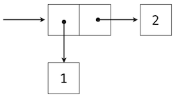
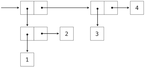
A standard way to visualize a pair --- in this case, the pair (1,2) --- is called box-and-pointer notation. Each value, compound or primitive, is depicted as a pointer to a box. The box for a primitive value contains a representation of that value. For example, the box for a number contains a numeral. The box for a pair is actually a double box: the left part contains (an arrow to) the first element of the pair and the right part contains the second.

This Python expression for a nested tuple

>>> ((1, 2), (3, 4))
((1, 2), (3, 4))

would have the following structure.

Our ability to use tuples as the elements of other tuples provides a new means of combination in our programming language. We call the ability for tuples to nest in this way a closure property of the tuple data type. In general, a method for combining data values satisfies the closure property if the result of combination can itself be combined using the same method. Closure is the key to power in any means of combination because it permits us to create hierarchical structures --- structures made up of parts, which themselves are made up of parts, and so on. We will explore a range of hierarchical structures in Chapter 3. For now, we consider a particularly important structure.

2.4.2   Recursive Lists

We can use nested pairs to form lists of elements of arbitrary length, which will allow us to implement the sequence abstraction. The figure below illustrates the structure of the recursive representation of a four-element list: 1, 2, 3, 4.

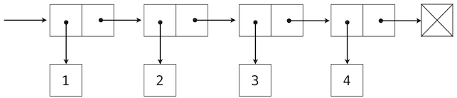
The list is represented by a chain of pairs. The first element of each pair is an element in the list, while the second is a pair that represents the rest of the list. The second element of the final pair is the empty tuple, which indicates that the list has ended, and is represented by a box with a cross through it. We can construct this structure using a nested tuple literal:

>>> (1, (2, (3, (4, ()))))
(1, (2, (3, (4, ()))))

This nested structure corresponds to a very useful way of thinking about sequences in general. A non-empty sequence can be decomposed into:

• its first element, and
• the rest of the sequence.

The rest of a sequence is itself a (possibly empty) sequence. We call this view of sequences recursive, because sequences contain other sequences as their second component.

Since our list representation is immutable and recursive, we will call it an IRList in our implementation, so as not to confuse it with the built-in list type in Python that we will introduce later in this chapter. A recursive list can be constructed from a first element and the rest of the list. The empty tuple represents an empty recursive list.

>>> empty_rlist = ()

>>> def make_irlist(first, rest=empty_irlist):
        """Make a recursive list from its first element and the rest
        (the empty immutable recursive list, by default)."""
        return (first, rest)

>>> def irlist_first(irlist):
        """Return the first element of the immutable recursive list irlist."""
        return irlist[0]

>>> def irlist_rest(irlist):
        """Return the rest of the elements of the immutable recursive list irlist."""
        return irlist[1]

These two selectors, one constructor, and one constant together implement the recursive list abstract data type. The single behavior condition for a recursive list is that, like a pair, its constructor and selectors are inverse functions.

• If a recursive list s was constructed from element f and list r, then irlist_first(s) returns f, and irlist_rest(s) returns r.

We can use the constructor and selectors to manipulate recursive lists.

>>> counts = make_irlist(1, make_irlist(2, make_irlist(3, make_irlist(4, empty_irlist))))
>>> irlist_first(counts)
1
>>> irlist_rest(counts)
(2, (3, (4, ())))

The recursive list can store a sequence of values in order, but it does not yet implement the sequence abstraction. Using the abstract data type we have defined, we can implement the two behaviors that characterize a sequence: length and element selection.

>>> def irlist_len(irlist):
        """Return the length of irlist."""
        if irlist == empty_irlist:
            return 0
        return 1 + irlist_len(irlist_rest(irlist))

>>> def irlist_select(irlist, index):
        """Return an item at the position index in irlist."""
        if index == 0:
            return irlist_first(irlist)
        return irlist_select(irlist_rest(irlist), index - 1)

Now, we can manipulate a recursive list as a sequence:

>>> irlist_len(counts)
4
>>> irlist_select(counts, 1)        # The second item has index 1.
2

Both of these implementations are recursive: Since IRLists are defined recursively, it seems natural to consider a recursive implementation of any function that operates on them. Each recursive call peels away each layer of the nested pair until the end of the list (in irlist_len) or the desired element (in irlist_select) is reached.

Here is another example of a function that operates recursively on a recursive list: We will define the function irlist_map, similar to the map function that we saw from before, which takes in a recursive list and a function to apply on the elements in the recursive list, and then returns a new recursive list that contains the results of applying the function on the elements in the original list. Notice that we have to construct a new recursive list since the original list is immutable, a property that the underlying tuple representation ensures.

>>> def irlist_map(func, irlist):
        if irlist == empty_irlist:
            return empty_irlist
        first = irlist_first(irlist)
        return make_irlist(func(first), irlist_map(func, irlist_rest(irlist)))

>>> my_irlist = make_irlist(1, make_irlist(2, make_irlist(3, make_irlist(4, empty_irlist)))))
>>> irlist_str(irlist_map(my_irlist))
"<1, 4, 9, 16>"

The above implementation first considers the simplest possible input, which is the empty recursive list. The result, in this case, is also the empty recursive list. However, if the list is not empty, then the function is called recursively on a shorter suffix that ignores the first element of the list. Assuming, as we do when thinking recursively, that this function call returns the correct result, we construct a new list whose first element is the result of applying the function to the first element of the original list; the rest of this new list is the result of the recursive call.

This example demonstrates a common pattern of computation with recursive lists, where each recursive call operates on an increasingly shorter suffix of the original list. This incremental processing to find the length and elements of a recursive list does take some time to compute. Python's built-in sequence types are implemented in a different way that does not have a large computational cost for computing the length of a sequence or retrieving its elements.

This example also introduces the new function irlist_str, which displays the contents of the recursive list. We use the angle brackets (< and >) to remind ourselves that the sequence is an immutable recursive list, and also that the implementation of the immutable recursive list is irrelevant to the functions that work with and operate on recursive lists. Recall that we were able to represent pairs using functions, and therefore we can represent recursive lists using functions as well, instead of using tuples. In both cases --- if the recursive list were represented using either tuples or functions --- we need only interact with the constructors and selectors, illustrating the power of data abstraction and the ability to separate implementation from usage.

The function irlist_str is defined here, as are other useful utility functions for working with recursive lists.

2.4.3   Dictionaries

Elements in IRLists and tuples are indexed by numbers. However, in many common situations, we would like to use more descriptive keys as our indices, especially when storing and manipulating correspondence relationships. The immutable dictionary (or IDict) allows us to use indices that are not necessarily numbers. For example, the following dictionary gives the values of various Roman numerals:

>>> numerals = make_idict(('I', 1), ('V', 5), ('X', 10))

The argument to the make_idict constructor function is a tuple of tuples, each of which is a key-value pair that maps a Roman numeral (a key) to its corresponding decimal number (a value). numerals is now a dictionary that maintains these key-value relationships, where both the keys and values are objects. The purpose of a dictionary is to provide an abstraction for storing and retrieving values that are indexed not by consecutive integers, but by descriptive keys. Strings commonly serve as keys, because strings are our conventional representation for names of things.

We can look up values by their keys using the idict_select function:

>>> idict_select(numerals, 'X')
10

If the key does not exist, the function returns None:

>>> idict_select(numerals, 'L')

No output is shown since the Python interpreter knows not to show the value None.

A dictionary can have at most one value for each key. Adding new key-value pairs and changing the existing value for a key can both be achieved using the idict_insert function, which returns the updated dictionary:

>>> numerals = idict_insert(numerals, 'L', 50)
>>> idict_str(numerals)
"('V' -> 5, 'X' -> 10, 'I' -> 1, 'L' -> 50)"
>>> numerals = idict_insert(numerals, 'I', 1)
>>> idict_str(numerals)
"('V' -> 5, 'X' -> 10, 'L' -> 50, 'I' -> 1)"

The idict_str function returns the contents of the dictionary as a string that shows the key and its corresponding value. The important thing to note from the output is that dictionaries, unlike the lexicographic product, are unordered collections of key-value pairs. When we print a dictionary, the keys and values are rendered in some order, but as users, we cannot predict what that order will be.

The dictionary abstraction also supports various methods of iterating of the contents of the dictionary as a whole. The methods idict_keys, idict_values and idict_items all return iterable values.

>>> idict_keys(numerals)
('V', 'X', 'L', 'I')
>>> idict_values(numerals)
(5, 10, 50, 1)
>>> sum(idict_values(numerals))
66
>>> idict_items(numerals)
(('V', 5), ('X', 10), ('L', 50), ('I', 1))

Dictionaries do have some restrictions:

• A key of a dictionary cannot be an object of a mutable built-in type.
• There can be at most one value for a given key.

This first restriction is tied to the underlying implementation of dictionaries. The details of this implementation are not a topic of this course. Intuitively, consider that the key tells Python where to find that key-value pair in memory; if the key changes, the location of the pair may be lost.

The second restriction is a consequence of the dictionary abstraction, which is designed to store and retrieve values for keys. We can only retrieve the value for a key if at most one such value exists in the dictionary.

The immutable dictionary ADT is defined here, as are useful utility functions for working with dictionaries.

2.4.4   Hierarchical Structures

Hierarchical structures result from the closure property of different data types, which asserts, for example, that tuples can contain other tuples. For instance, consider this nested representation of the numbers 1 through 4.

>>> ((1, 2), 3, 4)
((1, 2), 3, 4)

This tuple is a sequence of length three, of which the first element is itself a tuple. A box-and-pointer diagram of this nested structure shows that it can also be thought of as a tree with four leaves, each of which is a number.

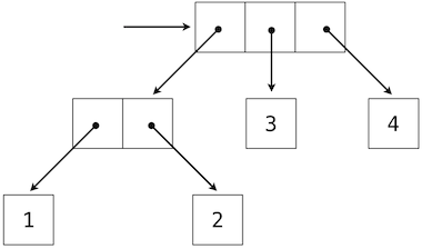
Like IRLists, this definition of a tree is naturally recursive. In a tree, each subtree is itself a tree. As a base case, any bare element that is not a tuple is itself a simple tree, but one with no branches and children. That is, the numbers are all trees, as is the pair (1, 2) and the structure as a whole.

For now, we will call these trees that only have items at the leaves deep tuples, since the term tree is usually reserved for a different structure we will see later in in a moment.

>>> def count_items(deep_tup):
        if type(deep_tup) != tuple:
            return 1
        return sum(map(count_items, deep_tup))

>>> dt = ((1, 2), 3, 4)
>>> count_items(dt)
4
>>> big_deep_tup = ((dt, dt), 5)
>>> big_deep_tup
((((1, 2), 3, 4), ((1, 2), 3, 4)), 5)
>>> count_items(big_deep_tup)
9

>>> def deep_map(deep_tup, fn):
        if type(deep_tup) != tuple:
            return fn(deep_tup)
        return tuple(deep_map(branch, fn) for branch in deep_tup)

>>> deep_map(big_deep_tup, square)
((((1, 4), 9, 16), ((1, 4), 9, 16)), 25)

>>> us_tree = make_itree("United States",
                         (make_itree("California",
                                     (make_itree("Los Angeles"),
                                      make_itree("San Francisco"),
                                      make_itree("Berkeley"))),
                          make_itree("New York",
                                     (make_itree("New York City"),
                                      make_itree("Ithaca"),
                                      make_itree("Buffalo"))),
                          make_itree("Texas",
                                     (make_itree("Austin"),
                                      make_itree("San Antonio"),
                                      make_itree("Dallas")))))
>>> itree_datum(us_tree)
"United States"
>>> tuple(map(itree_datum, itree_children(us_tree)))
("California", "New York", "Texas")

>>> print(itree_str(us_tree))
'United States'
|
+-'California'
| |
| +-'Los Angeles'
| |
| +-'San Francisco'
| |
| +-'Berkeley'
|
+-'New York'
| |
| +-'New York City'
| |
| +-'Ithaca'
| |
| +-'Buffalo'
|
+-'Texas'
  |
  +-'Austin'
  |
  +-'San Antonio'
  |
  +-'Dallas'

>>> from operator import add
>>> from functools import reduce
>>> def count_nodes(it):
        """Return the number of nodes in the ITree it."""
        return 1 + reduce(add, map(count_nodes, itree_children(it)), 0)

>>> count_nodes(us_tree)
13

>>> def itree_count_nodes(it):
        """Return the number of nodes in the ITree it."""
        return 1 + forest_count_nodes(itree_children(it))

>>> def forest_count_nodes(f):
        """Return the number of nodes in the forest (a tuple of trees) f."""
        if len(f) == 0:
            return 0
        return itree_count_nodes(f[0]) + forest_count_nodes(f[1:])

>>> itree_count_nodes(us_tree)
13

>>> def itree_map(fn, it):
        return make_itree(fn(itree_datum(it)),
                          tuple(itree_map(fn, child) for child in itree_children(it)))

>>> test_tree = make_itree(1, (make_itree(2, (make_itree(3),
                                              make_itree(4))),
                               make_itree(5, (make_itree(6),
                                              make_itree(7)))))
>>> print(itree_str(test_tree))
1
|
+-2
| |
| +-3
| |
| +-4
|
+-5
  |
  +-6
  |
  +-7

>>> print(itree_str(itree_map(lambda x: x * x, test_tree)))
1
|
+-4
| |
| +-9
| |
| +-16
|
+-25
  |
  +-36
  |
  +-49

>>> def contains(irl, item):
        """Returns True if item is a member of irl."""
        if irl == empty_irlist:
            return False
        return irlist_first(irl) == item or contains(irlist_rest(irl), item)

>>> contains(irlist_populate(4, 2, 3, 5, 1), 2)
True
>>> contains(irlist_populate(4, 2, 3, 5, 1), 66)
False

>>> empty_bst = None
>>> def make_bst(datum, left=make_itree(None), right=make_itree(None)):
        """Create a BST with datum, left branch, and right branch."""
        return (left, datum, right)

>>> def bst_datum(bst)
        """Return the datum of BST b."""
        return b[1]

>>> def bst_left(bst):
        """Return the left branch of BST b."""
        return b[0]

>>> def bst_right(bst):
        """Return the right branch of BST b."""
        return b[2]

>>> test_bst = make_bst(7,
                        left=make_bst(3,
                                      left=make_bst(1,
                                                    left=make_bst(0),
                                                    right=make_bst(2)),
                                      right=make_bst(5,
                                                     left=make_bst(4),
                                                     right=make_bst(6))),
                        right=make_bst(11,
                                       left=make_bst(9,
                                                     left=make_bst(8),
                                                     right=make_bst(10)),
                                       right=make_bst(13,
                                                      left=make_bst(12),
                                                      right=make_bst(14))))
>>> print(bst_str(test_bst))
7
|
+-3
| |
| +-1
| | |
| | +-0
| | |
| | +-2
| |
| +-5
|   |
|   +-4
|   |
|   +-6
|
+-11
  |
  +-9
  | |
  | +-8
  | |
  | +-10
  |
  +-13
    |
    +-12
    |
    +-14
>>> test_bst2 = make_bst(2, left=make_bst(1))
>>> print(bst_str(test_bst2))
2
|
+-1
|
+-empty_bst

>>> def bst_find(b, item):
        """Return True if item is in BST b and False otherwise."""
        if b == empty_bst:
            return False
        elif bst_datum(b) == item:
            return True
        elif bst_datum(b) > item:
            return bst_find(bst_left(b), item)
        return bst_find(bst_right(b), item)

>>> test_bst = make_bst(0,
                        left=make_bst(-4,
                                      left=make_bst(-6,
                                                    left=make_bst(-7),
                                                    right=make_bst(-5)),
                                      right=make_bst(-2,
                                                     left=make_bst(-3),
                                                     right=make_bst(-1))),
                        right=make_bst(4,
                                       left=make_bst(2,
                                                     left=make_bst(1),
                                                     right=make_bst(3)),
                                       right=make_bst(6,
                                                      left=make_bst(5),
                                                      right=make_bst(7))))
>>> bst_find(test_bst, 5)
True
>>> bst_find(test_bst, 22)
False
>>> bst_find(test_bst, 0.5)
False
>>> bst_find(test_bst, 1)
True

>>> lopsided = make_bst(6,
                        left=make_bst(5,
                                      left=make_bst(4,
                                                    left=make_bst(3))))
>>> print(bst_str(lopsided))
6
|
+-5
| |
| +-4
| | |
| | +-3
| | |
| | +-empty_bst
| |
| +-empty_bst
|
+-empty_bst