A. Intro: Balancing search trees

An Overview of Balanced Search Trees

Over the past couple of weeks, we have analyzed the performance of algorithms for access and insertion into binary search trees under the assumption that the trees were balanced. Informally, that means that the paths from root to leaves are all roughly the same length, and that we won't have to worry about lopsided trees in which search is linear rather than logarithmic.

This balancing doesn't happen automatically, and we have seen how to insert items into a binary search tree to produce worst-case search behavior. There are two approaches we can take to make tree balancing happen: incremental balance, where at each insertion or deletion we do a bit of work to keep the tree balanced; and all-at-once balancing, where we don't do anything to keep the tree balanced until it gets too lopsided, then we completely rebalance the tree.

In the activities of this segment, we start by analyzing some tree balancing code. Then we explore how much work is involved in maintaining complete balance. We'll move on to explore two kinds of balanced search trees, B trees and red-black trees.

B. B-trees

2-4 Trees

Let us examine 2-4 trees that guarantee O(log(n)) depth in any case. That is, the tree is always almost balanced.

In a 2-4 tree, also known as a 2-3-4 tree, each node can have up to 3 keys in it. The additional invariant is that any non-leaf node must have one more child than it does keys. That means that a node with 1 key must have 2 children, 2 keys with 3 children, and 3 keys with 4 children. That's why it's called a 2-3-4 tree.

Here's an example of one:

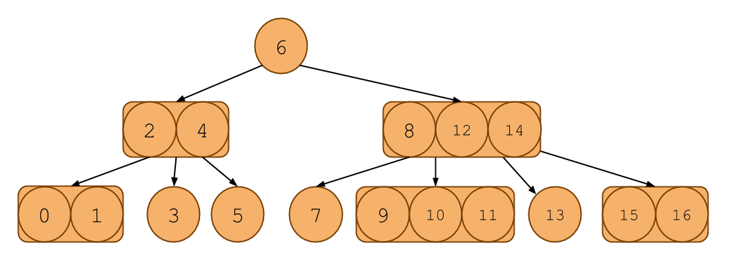
It looks like a binary search tree, except each node can contain 1, 2, or 3 items in it. Notice that it even follows the ordering invariants of the binary search tree.

Searching in a 2-4 tree is much like searching in a binary search tree. Like a BST, if there is only one key in a node, then everything to the left of the key is less than it and everything to the right is greater. If there are 2 keys, say A and B, then the leftmost child will all have keys less than or equal A, the middle child will have keys between A and B and the rightmost child will have keys greater than or equal to B. You can extend this to the 3 key case as well.

Insertion into a 2-4 Tree

Although searching in a 2-4 tree is like searching in a BST, inserting a new item is a little different.

First of all, we always insert the new key at the leaf node. We must find the correct place for the key that we insert to go, by traversing down the tree, then insert the new key in an appropriate place in the existing leaf.

For example, say we are inserting 10, and we traverse down the tree until we find a leaf with 2 other elements, 8, 11. Then, we can just insert 10 between 8 and 11, and the leaf now has three elements: 8, 10, 11.

However, what if we come across a node that already has 3 keys, such as 8, 9, and 11? We'd like to put the new item here, but it won't fit, because each node can only have up to 3 keys in it. What should we do?

Here, we do NOT add the item as a new child of the node. Instead, we add the key temporarily to the node, and push one of the middle keys (note that the choice of which middle key to push up is arbitrary, and will be clearly specified in any example we ask of you) up into the parent node and split the remaining two keys into two 1-key nodes (Because we are doing this from the top down, the parent will always have room). Then we add the new item to one of the split nodes.

For instance, say we had this 2-4 tree:

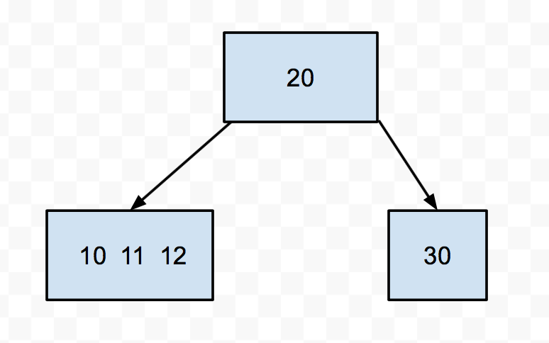
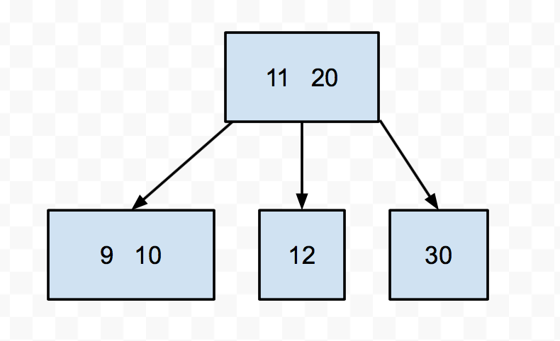
Let's try to insert 9 into this tree. We see it's smaller than 20, so we go down to the left. Then we find a node with 3 keys. We push up the middle (11), then split the 10 and the 12. Then we put the 9 in the appropriate split node.

There is one little special case we have to worry about when it comes to inserting, and that's if the root is a 3-key node. After all, roots don't have a parent. In that case, we still push up the middle key and instead of giving it to the parent, we make it the new root.

Self-test: Growing a 2-4 Tree

Suppose the keys 1, 2, 3, 4, 5, 6, 7, 8, 9, and 10 are inserted sequentially into an initially empty 2-4 tree. Which insertion causes the second split to take place? Assume we push up the left middle key when we try to insert into a node that is already full.

B-trees

A 2-4 tree is a special case of a structure called a B-tree. What varies among B-trees is the number of keys/subtrees per node. B-trees with lots of keys per node are especially useful for organizing storage of disk files, for example, in an operating system or database system. Since retrieval from a hard disk is quite slow compared to computation operations involving main memory, we generally try to process information in large chunks in such a situation, in order to minimize the number of disk accesses. The directory structure of a file system could be organized as a B-tree so that a single disk access would read an entire node of the tree. This would consist of (say) the text of a file or the contents of a directory of files.

C. Red-Black Trees

We have seen that B-trees are balanced, guaranteeing that a path from the root to any leaf is almost O(log(n)). However, B-trees are notoriously difficult and cumbersome to code, with numerous corner cases for common operations.

A Red-Black tree is a usual binary search tree, but it has additional invariants related to "coloring" each node red or black. This provides an isometry (one-to-one mapping) between 2-4 trees and Red-Black trees!

The conseqeunce is quite astounding: Red-Black trees maintain the balancedness of B-trees while inheriting all normal binary search tree operations (A Red-Black tree IS a binary search tree) with additional housekeeping. In fact, Java's java.util.TreeMap and java.util.TreeSet are implemented as Red-Black trees!

2-4 tree ↔ Red-Black tree

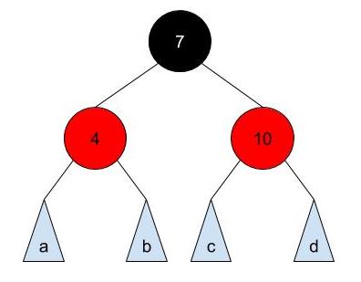
Notice that a 2-4 tree can have 1, 2, or 3 elements per node, and 2, 3, or 4 pointers to its children. Consider the following B-tree node:

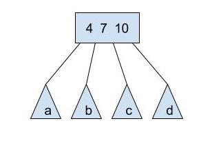
a, b, c, and d are pointers to its children nodes, therefore, its subtrees. a will have elements less than 4, b will have elements between 4 and 7, c will have elements between 7 and 10, and d will have elements greater than 10.

Let's transform this into a "section" in a Red-Black tree that represents the above node and its children pointers:

For each node in the 2-4 tree, we have a group of normal binary search tree nodes that correspond to it:

Middle element ↔ black node that is the right or left child of its parent node. Left element ↔ red node on the left of the black node. Right element ↔ red node on the right of the black node.

Notice that a, b, c, and d are also "sections" that correspond to a 2-4 tree node. Thus, the subtrees will have black root nodes.

How about a 2-4 node with two elements?

This node can be transformed as:

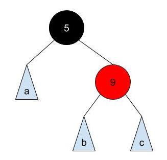
or

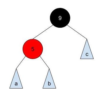
Both are valid. However, only the second transformation is a valid Left-Leaning Red-Black Tree, which we'll discuss in the next section.

Trivially, for 2-4 node with only one element, it will translate into a single black node in a Red-Black tree.

Convince yourself that the balancedness of the 2-4 tree still holds on a Red-Black tree and that the Red-Black tree is a binary search tree.

Exercise:

Read the code in RedBlackTree.java and BTree.java. Then, in RedBlackTree.java, fill in the implementation for buildRedBlackTree which returns the root node of the Red-Black tree which has a one-to-one mapping to a given 2-4 tree. For 2-4 tree node with 2 elements in a node, you must use the left element as the black node to pass the autograder tests. For the example above, you must use the first representation of Red-Black tree where 5 is the black node.

Red-Black trees are Binary Search Trees

As stated above, Red-Black trees are in fact binary search trees: a node's left subtree contains all elements less than that node's element and the same holds for the right subtree.

D. Left-Leaning Red-Black Trees (LLRB)

In the last section, we examined 2-4 trees their relationship to Red-Black trees. Here, we want to extend our discussion a little bit more and examine 2-3 trees and Left-Leaning Red-Black trees.

2-3 trees are B-trees, just like 2-4 trees. However, they can have up to 2 elements and 3 children, whereas 2-4 trees could have one more of each. Naturally, we can come up with a Red-Black tree counterpart. However, since we can only have nodes with 1 or 2 elements, we can either have a single black node (for a one-element 2-3 node) or a "section" with a black node and a red node (for a two-element 2-3 node). As seen in the previous section, we can either let the red node be a left child or a right child. However, we choose to always let the red node be the left child of the black node. This leads to the name, "Left-Leaning" Red-Black tree.

The advantages of the LLRB tree over the usual Red-Black tree is the ease of implementation. Since there are less special cases for each "section" that represents a 2-3 node, the implementation is much simpler.

Normal binary search tree insertions and deletions can break the Red-Black tree invariants, so we need additional operations that can "restore" the Red-Black tree properties. In LLRB trees, there are two key operations that we use to restore the properties: rotations and color flips.

Rotations

Consider the following tree:

   parent
     |
     7
   /   \
  1     c
 / \
a   b

a is a subtree with all elements less than 1, b is a subtree with elements between 1 and 7, and c is a subtree with all elements greater than 7. Now, let's take a look at another tree:

parent
  |
  1
 / \
a   7
   / \
  b   c

There are few key things to notice:

1. The root of the tree has changed from 7 to 1.
2. a, b, and c are still correctly placed. That is, their items do not violate the binary search tree invariants.
3. The height of the tree can change by 1.

Here, we call this transition from the first tree to the second a "right rotation on 7".

Now, convince yourself that a "left rotation on 1" on the second tree will give us the first tree. The two operations are symmetric, and both maintain the binary search tree property!

Discussion: Rotation by Hand

We are given an extremely unbalanced binary search tree:

    0
     \
      1
       \
        3
       / \
      2   6
         / \
        4   8

Write down a series of rotations (i.e. rotate right on 2) that will make tree balanced and have height of 2. HINT: Two rotations are sufficient.

Exercise: Rotation Implementation

Now we have seen that we can rotate the tree to balance it without violating the binary search tree invariants. Now, we will implement it ourselves! In RedBlackTree.java, implement rotateRight and rotateLeft. For your implementation, make the new root have the color of the old root, and color the old root red.

Hint: The two operations are symmetric. Should the code significantly differ?

Color Flip

Now we consider the color flip operation that is essential to LLRB tree implementation. Given a node, this operation simply flips the color of itself, and the left and right children. However simple it may look now, we will examine its consequences later on.

For now, take a look at the implementation provided in RedBlackTree.java.

Insertion

Finally, we are ready to put the puzzles together and see how insertion works on LLRB trees!

Say we are inserting x.

1. If the tree is empty, let x be the root with black color.
2. Do the normal binary search tree insertion, and color x red.
3. Restore LLRB properties.

Restoring LLRB Properties after Insertion.

First, let's assume that our new node x is the only child of a black node. That is:

     parent (black)
    /
   x (red)

or

   parent (black)
        \
         x (red)

Since we decided to make our tree left leaning, we know that the first tree is the valid form. If we end up with the second tree (x > parent) we can simply apply rotateLeft on parent to get the first tree.

Now, let's consider the case when our new node x becomes a child to a black node which already has a left child, or a child to a red node. Recall that LLRB has a one-to-one mapping to a 2-3 tree. This is like inserting x into a 2-3 tree node that already has 3 children!

Here, we have to deal with 3 different cases, and we will label them case A, B, C.

Case A: x ends up as the right child of the black node.

         |
         5(black)
     /      \
    1(red)   x(red)

Notice that for case A, the resulting section is the same as a 2-3 tree node with one extra element:

      |
   1  5  x

To fix it, we "split" the 2-3 node into two halves, "pushing" up the middle element to its parent:

        |
     5  (sibling)
   |  |         |
   1  x     (nephews)

Analogously, for our LLRB section, we can apply flipColor on 5. This results in:

      |
      5 (red)
  /      \
1(black)  x(black)

Notice that this exactly models the 2-3 node we desired. 5 is now a red node, which means that it is now part of the "parent 2-3 node section". Now, if 5 as a new red node becomes a problem, we can recursively deal with it as we are dealing with x now. Also, note that the root of the whole tree should always be black, and it is perfectly fine for the root to have two black children. It is simply a root 2-3 node with single element and two children, each with single element.

Case B: x ends up as the left child of the red node.

     |
     5 (black)
    /
   1 (red)
  /
 x (red)

In this case, we can apply rotateRight on 5, which will result in:

        |
        1 (black)
   /        \
  x(red)     5 (red)

This should look familiar, since it is exactly case A that we just examined before! After a rotation, our problem reduces to solving case A. Convince yourself that rotation performed here correctly handles the color changes and maintains the binary search tree properties.

Case C: x ends up as the right child of the red node.

          |
          5 (black)
       /
     1 (red)
      \
       x (red)

In this case, we can apply rotateLeft on 1, which will result in:

         |
         5 (black)
        /
       x (red)
      /
     1 (red)

This also should look familiar, since it is exactly case B that we just examined. We just need one more rotation and color flip to restore LLRB properties.

Exercise:

Now, we will implement insert in RedBlackTree.java. We have provided you with most of the logic structure, so all you need to do is deal with normal binary search tree insertion and handle case A, B, and C.

Discussion.

We have seen that even though the LLRB tree guarantees that the tree will be almost balanced, LLRB insert operation requires many rotations and color flips. Examine the procedure for the insertion and convince yourself and your partner that insert operation still takes O(log(n)) as in balanced binary search trees.

Hint: How long is the path from root to the new leaf? For each node along the path, are additional operations limited to some constant number? What does that mean?

Deletion

Deletion deals with many more corner cases and is generally more difficult to implement. For time's sake, deletion is left out for this lab.

E. Optional: Making a Balanced Tree

Exercise: Build a Balanced Tree from a Linked List

In BST.java complete the linkedListToTree method which should build a balanced binary search tree out of an already sorted LinkedList. Also, provide a good comment for the method linkedListToTree. Note that in the BST constructor, we pass in list.iterator() to linkedListToTree. What do we know about repeated calls to iter.next() given that the LinkedList is already sorted?

HINT: Recursion!

Question: If it's a BST, why are the items just of Object type? Why not Comparable?

Answer: Because you shouldn't need to ever do any comparisons yourself. Just trust that the order in the LinkedList is correct.

Self-test: linkedListToTree Speed

Give the runtime of linkedListToTree, where N is the length of the linked list. The runtime is in:

F. Conclusion

Summary

We hope you enjoyed learning about balanced search trees. They can be a bit tricky to implement compared to a normal BST, but the speedup in runtime helps us immensely in practice! Now that you've seen them, hopefully you can appreciate the work that went into Java's TreeMap and TreeSet that you can use as a black box.

Submission

Tag and push normally. Modified files should be RedBlackTree.java and, optionally, BST.java.