Project 2: CS61Classify

Overview

Part A Due Wednesday, October 16th

Part B Due Wednesday, October 23rd

The purpose of this project is to have you implement a simple, yet extremely useful system in RISC-V assembly language. You will learn to use registers efficiently, write functions, use calling conventions for calling your functions, as well as external ones, allocate memory on the stack and heap, work with pointers and more!

To make the project more interesting, you will implement functions which operate on matrices and vectors – for example, matrix multiplication. You will then use these functions to construct a simple Artificial Neural Net (ANN), which will be able to classify handwritten digits to their actual number! You will see that ANNs can be simply implemented using basic numerical operations, such as vector inner product, matrix multiplications, and thresholding.

Getting Started

You will be working with partners for this project, which means the two of you will be sharing the same GitHub repository. To pull the starter code, first accept the GitHub Classroom assignment and clone the repo that’s been created for your team. Then, from within that cloned repository, add the starter code repo as a remote repository in git and pull the starter code.

git clone YOUR_REPO_NAME
cd YOUR_REPO_NAME
git remote add starter https://github.com/61c-teach/fa19-proj2-starter.git
git pull starter master

You’ll need both Java and Python 3 for this project, which we assume you have from CS61A and CS61B. If not, these CS61A and CS61B setup instructions should help. Feel free to skip the steps that aren’t relevant.

Neural Networks

At a basic level, a neural networks tries to approximate a (non-linear) function that maps your input into a desired output. A basic neuron consists of a weighted linear combination of the input, followed by a non-linearity – for example, a threshold. Consider the following neuron, which implements the logical AND operation:

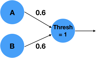
It is easy to see that for $A=0$, $B=0$, the linear combination $0*0.6 + 0*0.6 = 0$, which is less than the threshold of 1 and will result in a 0 output. With an input $A=0$, $B=1$ or $A=1$, $B=0$ the linear combination will results in $1*0.6 + 0*0.6 = 0.6$, which is less than 1 and result in a 0 output. Similarly, $A=1$, $B=1$ will result in $1*0.6+1*0.6=1.2$, which is greater than the threshold and will result in a 1 output! What is interesting is that the simple neuron operation can also be described as an inner product between the vector $[A,B]^T$ and the weights vector $[0.6,0.6]^T$ followed by as thresholding, non-linear operation.

More complex functions can not be described by a simple neuron alone. We can extend the system into a network of neurons, in order to approximate the complex functions. For example, the following 2 layer network approximates the logical function XOR:

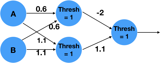
The above is a 2 layer network. The network takes 2 inputs, computes 2 intemediate values, and finally computes a single final output.

It can be written as matrix multiplications with matrices m_0 and m_1 with thresholding operations in between as shown below:

Convince yourself that this implements an XOR for the appropriate inputs!

You are probably wondering how the weights of the network were determined? This is beyond the scope of this project, and we would encourage you to take advanced classes in numerical linear algebra, signal processing, machine learning and optimization. We will only say that the weights can be trained by giving the network pairs of correct inputs and outputs and changing the weights such that the error between the outputs of the network and the correct outputs is minimized. Learning the weights is called: “Training”. Using the weights on inputs is called “Inference”. We will only perform inference, and you will be given weights that were pre-trained by your dedicated TA’s.

Handwritten Digit Classification

In this project we will implement a similar, but slightly more complex network which is able to classify handwritten digits. As inputs, we will use the MNIST data set, which is a dataset of 60,000 examples presented as images sized 28x28 = 784 pixels. These contain handwritten digits ranging from 0-9. We will treat these images as “flattened” input vectors sized 784x1. In a similar way to the example before, we will perform matrix multiplications with matrices m_0 and m_1, which have been pre-trained and will be given to you. Instead of thresholding we will use two different non-linearities: The ReLU and ArgMax functions. Details about these will be provided below. The network will then return a number representing the digit in the image. Here’s a schematic of the network:

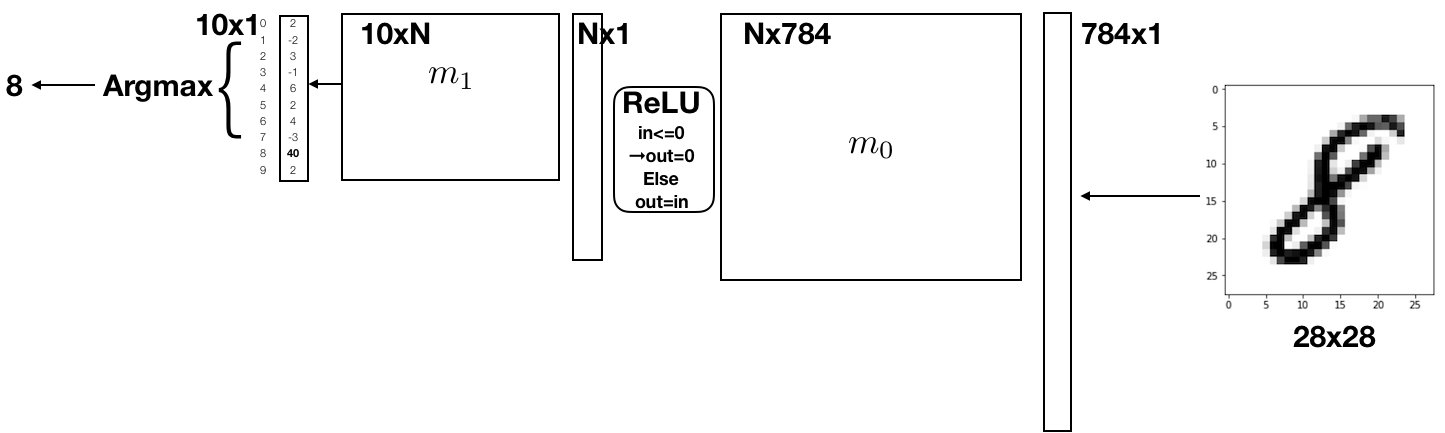
You will be required to implement the classification process by implementing matrix multiplication functions, the ReLU function and the ArgMax function. Putting these together, you will implement an ANN in RISC-V Assembly!

Running RISC-V in Venus

All the code you write will be in RISC-V, and will be run in Venus. There are two ways to run your code with Venus, either through the web interface or from the command line using a Java .jar file. We recommend that you do most of your development locally with the .jar file, and only use the web interface for debugging or making changes to one file at a time.

Method 1: Web Interface

The first option is to run Venus in your browser via a web interface, linked here. This web interface allows for easy debugging and editing of your code. It also has its own virtual filesystem, from which you can upload and download files. You can also switch between editing multiple files in the virtual filesystem and save the files you’re working on.

There are three tabs in the web interface:

• “Venus”, which gives you access to the Venus’ virtual terminal and filesystem
• “Editor”, which allow you to write and edit code
• “Simulator”, which allows you to run your code, and debug it by setting breakpoints, checking register values, and inspecting memory locations

Virtual Terminal and Filesystem

The “Venus” tab allows you to access the terminal, as well as Venus’ own filesystem. The terminal in Venus supports a specific set of commands. To see full list you can run help, but we’ve included some of the most important ones below.

• save <FILENAME>: Saves the code currently in the editor to FILENAME, creating/overwriting it as needed
• edit <FILENAME>: Copies the code in FILENAME into the editor. This will overwrite everything currently in the editor, so make sure to save as needed beforehand. Additionally, if you’ve used this command to open a file in the editor, you can then use Ctrl+S to quickly save your code back to the same file, instead of switching back to the terminal and using the save command.
• upload: Opens up a window allowing you to pick files from your local machine to upload to Venus
• download <FILENAME>: Opens up a window allowing you to download FILENAME to your local machine
• unzip <ZIP_FILENAME>: Unzips a .zip file into the current working directory.
• zip <ZIP_FILENAME> <FILENAME_1> <FILENAME_2> ... : Opens up a window allowing you to download a zip file called ZIP_FILE_NAME, which contains all the specified files and/or folders. Folders are added to the zip file recursively.

When uploading files to the Venus web interface, you’ll want to zip your entire project directory locally, use the upload in the Venus terminal to upload that zip file, and then unzip to retrieve all your project files.

Alternatively, you can upload individual files to work with. However, you’ll need to make sure the directory structure is the same as the starter repo, or be prepared to edit the relative paths given to you in the starter code for inputs and .import statements.

Note: We HIGHLY recommend that you regularly copy the changes you’ve made in the Venus web interface to your local machine to save them. If you accidentally close the browser window or run edit before running save, you could lose a large amount of progress. This is one of the primary reasons we recommend running with the .jar file for most of your development, and only turning to Venus to debug one specific file at a time.

Debugging in Venus

The “Simulator” tab allows you to view register/memory values, and set breakpoints for debugging. There are two ways to set breakpoints in the web interface. One way is to open up the simulator tab, assemble the code, and then click a line to set a breakpoint before running the program.

You can also use the ebreak command, which will set a break point at the following instruction. For example, in the following code, we’ve used ebreak to set a breakpoint on the line add t1 t0 1.

    addi t0 x0 1
    ebreak
    add t1 t0 1 # Debugger will stop right before this instruction
    add t2 t0 1

You can also use ebreaks alongside branch statements for conditional breakpoints. For example, let’s say you want to break only when t0 is equal to 0, and skip over the breakpoint otherwise. We could use ebreak in the following way to skip the breakpoint if t0 != 0.

    bne t0 x0 skip_break
    ebreak

skip_break:
    addi x0 x0 0
    addi t4 x0 3

Venus Settings: Mutable Text and the Tracer

One more thing you should know about are the settings in the “Venus” tab. Here you can do things like disable mutable text to catch bugs with altering the code portion of memory, set command line arguments to your program, as well as various other options. By default memory accesses between the stack and heap are disabled, but mutable text is allowed.

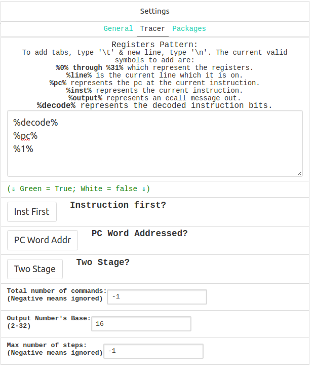
You can also enable tracing your program in the “Tracer” subtab of the settings tab. The tracer allows you to basically print out specific values on every step of your program. You can denote the values to be printed out in the text box under “Register Pattern”, as well as their format in the options below.

For example, the following settings will enable you to print the instruction itself as well as the registers pc and x1 in hexadecimal (base 16) on every step of your program:

Then, in the “Simulator” tab, if you click “Trace” instead of “Run” you’ll get the following printed output:

auipc x8 65536
00000004
00000000
addi x8 x8 0
00000008
00000000
...

Method 2: .jar file

The alternative way to run Venus is by running it as a Java .jar file, which we’ve provided for you as part of the starter code as venus.jar. If you want to download the latest version yourself, you can find it here or in the “JVM” subtab under the “Editor” tab in the web interface.

The .jar file runs much faster than the web interface, and will be the difference between your code taking several minutes vs. several seconds when we get to larger inputs. The downside is that you lose access to the debugging UI the web interface provides.

The basic command to run a given RISC-V file is as follows: java -jar venus.jar <FILENAME>

Note that if you’re getting an error about max instruction count being reached for large MNIST inputs, you can increase the instruction count with the -ms flag. Setting the max instruction count to a negative value will remove the limit altogether. java -jar venus.jar -ms -1 <FILENAME>

There are also various other flags, and you can see a complete list by running: java -jar venus.jar -h Like with the web version, you can disable mutable text with the -it flag.

Overall, we recommend you debug your code on smaller inputs via the web interface, and switch to the .jar version when running on larger, MNIST inputs. Note that you can also debug in the .jar version by using print functions like print_int and print_int_array, which are provided for you in utils.s.

Using the Tracer with the .jar file

You can also actually enable the tracer mentioned previously when using the .jar file as well. This can be done using the command line flag -t, after which you can use -tf to read in the pattern to print from a text file or -tp to read the pattern from the command line. You can also use the -tb command to specify the base of the register output.

For example, the following command will print out the instruction as well as the registers pc and x1 in hexadecimal (base 16) for every step of your program, and is equivalent to how we ran the tracer in the web interface previously.

java -jar venus.jar  <FILENAME> -t -tb 16 -tp "%decode%\n%pc%\n%x1%\n"

Testing Framework

In the test_files subdirectory, you’ll find several RISC-V files to test your code with. There is a test file corresponding to every function you’ll have to write, except for the main function in the final part of the project.

Some of these test files have been provided for you in their entirety, and you’ll only have to edit them to change their inputs. Other ones just include starter code, and have been left for you to fill out.

We will not be grading you on the tests you write for your own code. However, the autograder for this project will only give you basic sanity checks, and is not meant to be comprehensive. Instead, it is up to you to test your own functions, using both provided and self-written tests.

The goal of this is to help you build confidence in your own code in the absence of an autograder by writing your own tests.

RISC-V Calling Convention

We will be testing all of your code on RISC-V calling conventions, as described in lecture/lab/discussion. All functions that overwrite registers that are preserved by convention must have a prologue and epilogue where they save those register values to the stack at the start of the function and restore them at the end.

Following these calling conventions is extremely important for this project, as you’ll be writing functions that call your other functions, and maintaining the abstraction barrier provided by the conventions will make your life a lot easier.

We’ve provided # Prologue and # Epilogue comments in each function as a reminder. Note that depending on your implementation, some functions won’t end up needed a prologue and epilogue. In these cases, feel free to delete/ignore the comments we’ve provided.

For an closer look at RISC-V calling conventions, we’ve provided some excellent notes written by a former head TA for the course here.

Common Errors

• Ran for more than max allowed steps!: Venus will automatically terminate if your program runs for too many steps. This is expected for large MNIST sized inputs, and you can workaround it with the -ms flag. If you’re getting this for small inputs, you might have an infinite loop.
• Attempting to access uninitialized memory between the stack and heap.: Your code is trying to read or write to a memory address between the stack and heap pointers, which is causing a segmentation fault. Check that you’re allocating enough memory, and that you’re accessing the correct addresses.

Part A: Mathematical Functions

Due Monday, October 14th

In this part, you will implement some of matrix operations used by neural networks. These include a dot product, matrix multiplication, an elementwise ReLU, and a max function.

Background Knowledge

Matrix Format

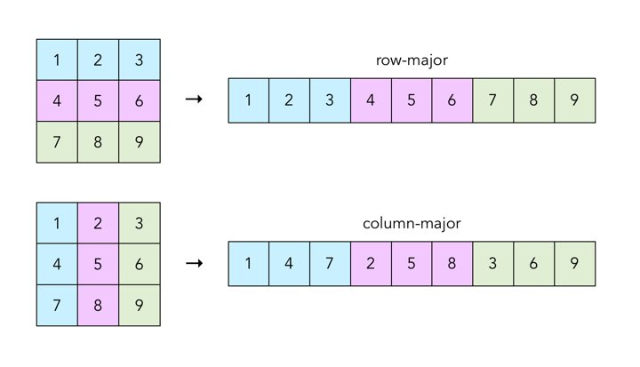
In this project, all two-dimensional matrices will be stored as a one-dimensional vector in row-major order. This should be a bit familiar, as it is the same representation we used for the output matrix in the Mandelbrot function in Project 1.

One way to think about it is that we can create a 1D vector from a 2D matrix by concatenating together all the rows in the matrix. Alternatively, we could concatenate all the columns together instead, which is known as column-major order.

For a more in-depth look at row-major vs. column-major order, see this Wikipedia page.

Vector/Array Strides

The stride of a vector is the number of memory locations between consecutive elements of our vector, measured in the size of our vector’s elements. If our stride is $n$, then the memory addresses of our vector elements are $n$ * sizeof(element) bytes apart.

So far, all the arrays/vectors we’ve worked with have had stride 1, meaning there is no gap betwen consecutive elements. Now, to do the row * column dot products with our row-major matrices that we’ll need for matrix multiplication, we will need to consider vectors with varying strides. Specifically, we’ll need to do this when considering a column vector in a flattened, row-major representation of a 2D matrix

Let’s take a look at a practical example. We have the vector int *a with 3 elements.

• If the stride is 1, then our vector elements are *(a), *(a + 1), and *(a + 2), in other words a[0], a[1], and a[2].
• However, if our stride is 4, then our elements are at *(a), *(a + 4), and *(a + 8) or in other words a[0], a[4], and a[8].

To summarize in C code, to access the ith element of a vector int *a with stride s, we use *(a + i * s), or a[i * s]. We leave it up to you to translate this memory access into RISC-V.

For a closer look at strides in vectors/arrays, see this Wikipedia page.

Task 1: ReLU

In relu.s, implement our relu function to apply the mathematical ReLU function on every element of the input array. This ReLU function is defined as $\text{ReLU}(a) = max(a, 0)$, and applying it elementwise on our matrix is equivalent to setting every negative value equal to 0.

An important thing to note is that this function, unlike most of the other functions in this project, will be performanced in-place. In other words, we won’t write to an output matrix, but instead directly change the values of the input matrix in memory. As a result, you’ll see that the relu function doesn’t take in an output matrix as an argument.

Additionally, notice that our relu function operates on a 1D vector, not a 2D matrix. We can do this because we’re applying the function individually on every element of the matrix, and our 2D matrix is stored in memory as a row-major 1D vector.

Testing: ReLU

We’ve provided test_relu.s for you to test your relu function. In it, you can set the values and dimensions of a matrix in static memory. Running the file will print that matrix before and after calling your relu function on it.

Task 2: ArgMax

Near the end of our neural net, we’ll be provided with scores for every possible classification. For MNIST, we’ll be given a vector of length 10 containing scores for every digit ranging from 0 to 9. The larger the score for a digit, the more confident we are that our handwritten input image contained that digit. Thus, to classify our handwritten image, we pick the digit with the highest score.

The score for the digit $i$ is stored in the $i$-th element of the array, to pick the digit with the highest score we find the array index with the highest value. In argmax.s, implement the argmax function to return the index of the largest element in the array. If there are multiple largest elements, return the smallest index.

Additionally, note that just like relu, this function takes in a 1D vector and not a 2D matrix. The index you’re expected to return is the index of the largest element in this 1D vector.

Testing: Argmax

We’ve provided test_argmax.s for you to test your argmax function. You can edit it to set a static vector v0 along with its length, and then run the file to print the output returned by running your function, which should be the index of the largest element in v0.

Task 3.1: Dot Product

In dot.s, implement the dot function to compute the dot product of two integer vectors. The dot product of two vectors $a$ and $b$ is defined as $dot(a, b) = \sum_{i=0}^{n-1} a_ib_i = a_0 * b_0 + a_1 * b_1 + \cdots + a_{n-1} * b_{n-1}$, where $a_i$ is the $i$th element of $a$.

Notice that this function takes in the a stride as a variable for each of the two vectors, make sure you’re considering this when calculating your memory addresses. We’ve described strides in more detail in the background section above, which also contains a detailed example on how stride affects memory addresses for vector elements.

Also note that we do not expect you to handle overflow when multiplying. This means you won’t need to use the mulh instruction.

For a closer look at dot products, see this Wikipedia page.

Testing: Dot Product

This time, you’ll need to fill out test_dot.s, using the starter code and comments we’ve provided. Overall, this test should call your dot product on two vectors in static memory, and print the result. Feel free to look at test_argmax.s and test_relu.s for reference.

By default, in the starter code we’ve provided, v0 and v1 point to the start of an array of the integers 1 to 9, continuous in memory. Let’s assume we set the length and stride of both vectors to 9 and 1 respectively. We should get the following:

v0 = [1, 2, 3, 4, 5, 6, 7, 8, 9]
v1 = [1, 2, 3, 4, 5, 6, 7, 8, 9]
dot(v0, v1) = 1 * 1 + 2 * 2 + ... + 9 * 9 = 285

What if we changed the length to 3 and the stride of the second vector v1 to 2, without changing the values in static memory? Now, the vectors contain the following:

v0 = [1, 2, 3]
v1 = [1, 3, 5]
dot(v0, v1) = 1 * 1 + 2 * 3 + 3 * 5 = 22

Note that v1 now has stride 2, so we skip over elements in memory when calculating the dot product. However, the pointer v1 still points to the same place as before: the start of the sequence of integers 1 to 9 in memory.

Task 3.2: Matrix Multiplication

Now that we have a dot product function that can take in varying strides, we can use it to do matrix multiplication. In matmul.s, implement the matmul function to compute the matrix multiplication of two matrices.

The matrix multiplication of two matrices $A$ and $B$ results in the output matrix $C = AB$, where $C[i][j]$ is equal to the dot product of the $i$-th row of $A$ and the $j$-ith column of $B$. Note that if we let the dimensions of $A$ be $(n*m)$, and the dimensions of $B$ be $(m * k)$, then the dimensions of $C$ must be $(n * k)$. Additionally, unlike integer multiplication, matrix multiplication is not commutative, $AB$ != $BA$.

Documentation on the function has been provided in the comments. A pointer to the output matrix is passed in as an argument, so you don’t need to allocate any memory for it in this function. Additionally, note that m0 is the left matrix, and m1 is the right matrix.

Note that since we’re taking the dot product of the rows of m0 with the columns of m1, the length of the two must be the same. If this is not the case, you should exit the program with exit code 2. This code has been provided for you under the mismatched_dimensions label at the bottom of the file, so all you need to do is jump to that label when the a row of m0 and a column of m1 do not have the same length.

A critical part of this function, apart from having a correctly implemented dot product, is passing in the correct row and column vectors to the dot product function, along with their corresponding strides. Since our matrices are in row-major order, all the elements of any single row are contiguous to each other in memory, and have stride 1. However, this will not be the case for columns. You will need to figure out the starting element and stride of each column in the right matrix.

For a closer look at matrix multiplication, see this Wikipedia page.

Testing: Matrix Multiplication

Fill out the starter code in test_matmul.s to test your matrix multiplication function. The completed test file should let you set the values and dimensions for two matrices in .data as 1D vectors in row-major order. When ran, it should print the result of your matrix multiplication.

Note that you’ll need to allocate space for an output matrix as well. The starter code does this by creating a third matrix in static memory.

For testing complicated inputs, you can use any available tool to help you calculate the expected output (numpy, wolfram, online matrix calculator).

m0 = [1, 2, 3
      4, 5, 6,
      7, 8, 9]
m1 = [1, 2, 3
      4, 5, 6,
      7, 8, 9]
matmul(m0, m1) =
     [30, 36, 42
      66, 81, 96
      102, 126, 150]

Part B: File Operations and Main

Due Monday, October 21th

In this part, you will implement functions to read matrices from and write matrices to binary files. Then, you’ll write a main function putting together all of the functions you’ve written so far into an MNIST classifier, and run it using pretrained weight matrices that we’ve provided.

Background Knowledge

Matrix File Format

Our matrix files come in two forms: binary and plaintext. We’ve included a python script called convert.py to convert between the two. The usage is as follows:

• python convert.py file.bin file.txt --to-ascii to go from binary to plaintext
• python convert.py file.txt file.bin --to-binary to go from plaintext to binary

Note that these commands assume your default Python version is Python 3. If you’re getting an error, you can run with Python 3 explicitly:

• python3 convert.py file.bin file.txt --to-ascii
• python3 convert.py file.txt file.bin --to-binary

Plaintext Format

The first line of the plaintext file will contain two integers, representing number of rows and columns of the matrix. Every line afterwards is a row of the matrix. For example, a plaintext file containing a 3x3 matrix would look like this:

3 3
1 2 3
4 5 6
7 8 9

Note that there is a newline after the final row of the matrix.

Binary Format

The first 8 bytes of the binary file represent two 4 byte integers. These integers are the number of rows and columns of the matrix. Every 4 following bytes represents an integer that is an element of the matrix, in row-major order. There are no gaps between elements.

Viewing Binary Files

If you simply open up a binary file with vim or any text editor, it would attempt to interpret the individual bytes as characters. This will result in an incomprehensible output.

There are a variety of ways to view binary files, but we recommend the xxd command. You can find it’s man page here, but its default functionality is to output the raw bits of the file in a hex representation.

Note that you can also use hexdump, but the ordering/endianness of bytes will be different. The following examples all assume you’re using xxd.

For example, let’s say the plaintext example in the previous section is stored in file.txt. We can run python convert.py file.txt file.bin --to-binary to convert it to a binary format, then xxd file.bin, which should print the following:

00000000: 0300 0000 0300 0000 0100 0000 0200 0000  ................
00000010: 0300 0000 0400 0000 0500 0000 0600 0000  ................
00000020: 0700 0000 0800 0000 0900 0000            ............

If you interpret this output 4 bytes at a time (equivalent to 8 hex digits) in little-endian order (see below), you’ll see that they correspond to the values in the plaintext file. Don’t forget that the first and second 4 bytes are integers representing the dimensions, and the rest are integer elements of the matrix.

Endianness

It is important to note that the bytes are in little-endian order. This means the least significant byte is placed at the lowest memory address. For files, the start of the file is considered the “lower address”. This relates to how we read files into memory, and the fact that the start/first element of an array is usually at the lowest memory address.

Practically, this means if we have the integer 3 corresponding to the hex 0x00 00 00 03, we’ll get 03 00 00 00 when we print the file with xxd. The bytes are reordered such that the least significant byte comes first.

RISC-V uses little-endian by default, and our files are all little-endian as well. This means you should never have to worry about endianness when writing code. Rather, it’s something you’ll need to keep in mind when debugging/viewing the bits.

Ecalls and Utils.s

The ecall instruction is a special command in RISC-V, and corresponds to a environment/system call. It has a broad range of functionality, involving reading/writing to files, printing to the command line, and exiting the program. For this project, we’ve created helper functions in utils.s that wrap around the various different ecalls for you to use. Do not make ecalls directly in your own code. Use these helper functions instead.

All of these functions are documented in inline comments in utils.s, alongside their arguments and return values. The most important of these are highlighted below.

• print_int, print_str, and print_char for printing values
• fopen, fread, fwrite, and fclose for reading/writing to files
• exit to quit the program with a zero exit code (no error)
• exit2 to quit the program with the integer in a1 as the exit code

Note that these ecall wrappers do not use a0 as input, because the ecall instruction itself uses it to denote which kind of ecall to make.

Additionally, there are two other helper functions you’ll find useful:

• malloc, which allocates a0 bytes on the heap, and returns a pointer to them in a0.
• print_int_array, which prints out all elements of an integer array

Note that there is no free helper function to go with malloc. For this project, and this project ONLY, you will not be required to free your malloc’ed memory.

File Operations

In the section above, we described the helper functions fopen, fread, fwrite, and fclose. Because these functions are critical for the read_matrix and write_matrix functions you’ll need to write, we’re going to explore them in depth here.

fopen

Opens a file that we can then read and/or write to, depending on the permission bit. Returns a file descriptor, which is a unique integer tied to the file. Must be called on a file before any other operations can be done on it.

• Arguments:
  • a1 is a pointer to a string containing the filename of the file to open
  • a2 is an integer denoting the permissions we open the file with. For example, we can open the file with read permissions, which prevents us from writing to it. For this project, we only really care about a few basic permission bits: 0, which corresponds to r for read only permission, and 1 which corresponds to w for write only permission. Note that w will overwrite the file if it already exists, and create it if it doesn’t.
• Return Values
  • a0 is a file descriptor, which is a unique integer tied to the file. We will call future file-related functions on this file descriptor, so we know which opened file we’re reading/writing/closing. On failure, a0 is set to -1.

fread

Reads a given number of bytes from a file into a buffer, which is a preallocated chunk of memory to store the bytes. Note that repeated reads will read consecutive bytes from the file. For example, two freads of 8 bytes on a file will read the first 8 bytes and then the second 8 bytes. It will not read the same 8 bytes twice.

• Arguments:
  • a1 is the file descriptor of the file we want to read from, previously returned by fopen.
  • a2 is a pointer to the buffer that we’re going to read the bytes from the file into. This must be an appropriate amount of memory that was allocated before calling the function, and passed in as a pointer.
  • a3 is the number of bytes to read from the file.
• Return Values
  • a0 is the number of bytes actually read from the file. If a0 != a3, then we either hit the end of the file or there was an error.

fwrite

Writes a given number of elements of a given size. Like fread, subsequent writes to the same file do not overlap, but are rather appended to each other. Note that unlike fread, we don’t pass in the total number of bytes but rather the total number of elements and the size of each element in bytes. We can multiply the two to find the total number of bytes written.

Additionally, note that our writes aren’t actually saved until we run fclose or fflush.

• Arguments:
  • a1 is the file descriptor of the file we want to write to, previously returned by fopen.
  • a2 is a pointer to a buffer containing what we want to write to the file.
  • a3 is the number of elements to write out of the buffer
  • a4 is the size of each buffer element in bytes
• Return Values
  • a0 is the number of elements actually written to the file. If a0 != a3, then we either hit the end of the file or there was an error.

fclose

Closes the file once we’re done with it, saving any writes we’ve made to it.

• Arguments:
  • a1 is the file descriptor of the file we want to close to, previously returned by fopen.
• Return Values
  • a0 is 0 on success, and -1 otherwise.

Task 1: Read Matrix

In read_matrix.s, implement the read_matrix function which uses the file operations we described above to read a binary matrix file into memory. If any file operation fails or doesn’t return the expected number of bytes, exit the program with exit code 1. The code to do this has been provided for you, simply jump to the eof_or_error label at the end of the file.

Recall that the first 8 bytes contains the two 4 byte dimensions of the matrix, which will tell you how many bytes to read from the rest of the file. Additionally, recall that the binary matrix file is already in row-major order.

You’ll need to allocate the memory for the matrix in this function as well. This will require a call to malloc, which is in util.s and also described in the background section above.

Finally, note that RISC-V only allows for a0 and a1 to be return registers, and our function needs to return three values: The pointer to the matrix in memory, the number of rows, and the number of columns. We get around this by having two int pointers passed in as arguments. We set these integers to the number of rows and columns, and return just the pointer to the matrix.

Testing: Read Matrix

Testing this function is a bit different from testing the others, as the input will need to be a properly formatted binary file that we can read in.

We’ve provided a skeleton for test_read_matrix.s, which will read the file test_input.bin, and then print the output. The file test_input.bin is the binary format of the plaintext matrix file test_input.txt. To change the input file read by the test you’ll need to edit test_input.txt first, then run the convert.py script with the --to-binary flag to update the binary.

From the root directory, it should look something like this: python convert.py --to-binary test_files/test_input.txt test_files/test_input.bin After this, you can run the test again, and it’ll read your updated test_input.bin.

Another thing to note is that you’ll need to allocate space for two integers, and pass in those memory addresses as arguments to read_matrix. You can do this either with malloc or by allocating space on the stack.

Task 2: Write Matrix

In write_matrix.s, implement the write_matrix function which uses the file operations we described above to write from memory to a binary matrix file. The file must follow the format described in the background section above. Like with read_matrix, exit the program with exit code 1 if any file operation fails or doesn’t return the expected number of bytes. You can do this by jumping to the provided eof_or_error label.

Testing: Write Matrix

For this function, instead of checking a printed output, you’ll need to check the file that was written. We’ve provided a skeleton for test_write_matrix.s, which should call your function to write a matrix stored in static .data to test_output.bin.

You can change what gets written by editing test_write_matrix.s, but to check that the output is correct you’ll need to interpret a binary format matrix file. This can be done either by converting it to plaintext with: python convert.py --to-ascii test_files/test_output.bin test_files/test_output.txt, or by manually inspecting the bits themselves with: xxd test_files/test_output.bin.

Task 3: Putting it all Together

In main.s, implement the main function. This will bring together everything you’ve written so far, and create a basic sequence of functions that will allow you to classifiy the preprocessed MNIST inputs using the pretrained matrices we’ve provided.

Note that for THIS PROJECT/FUNCTION ONLY, we will NOT require you to follow RISC-V calling convention by preserving saved registers in the main function. This is to make testing the main function easier, and to reduce its length. Normally, main functions do follow convention with a prologue and epilogue.

Command Line Arguments and File Paths

The filepaths for the input, m0, m1, and the output to write to will all be passed in on the command line. RISC-V handles command line arguments in the same way as C, at the start of the main function a0 and a1 will be set to argc and argv respectively.

We will call main.s in the following way: java -jar venus.jar main.s -it -ms -1 <M0_PATH> <M1_PATH> <INPUT_PATH> <OUTPUT_PATH>

Note that this means the pointer to the string M0_PATH will be located at index 1 of argv, M1_PATH at index 2, and so on.

If the number of command line arguments is different from what is expected, you code should exit with exit code 3. This will require a call to a helper function in utils.s. Take a look at the starter code for matmul, read_matrix, and write_matrix for hints on how to do this.

The Network

The first thing you’ll need to do (after verifying the number of command line arguments) is load m0, m1, and the input matrices into memory by making multiple calls to read_matrix, using command line arguments. Remember you need to pass in two integer pointers as arguments.

Next, you’ll want to use those three matrices to calculate the scores for our input. Our network consists of a matrix multiplication with m0, followed by a relu on the result, and then a second matrix multiplication with m1. At the end of this, we will have a matrix of scores for each classification. We then pick the index with the highest score, and that index is the classification for our input.

Given two weight matrices m0 and m1, along with an input matrix input, the pseudocode to generate the scores for each class is as follows:

hidden_layer = matmul(m0, input)
relu(hidden_layer) # Recall that relu is performed in-place
scores = matmul(m1, hidden_layer)

Once you’ve obtained the scores, we expect you to save them to the output file passed in on the command line. Then, call argmax, which will return a single integer representing the classification for your input, and print it.

Note that when calling argmax and relu, you should treat your inputs as 1D arrays. That means the length you pass into the function should be the number of elements in your entire matrix.

Testing main

All test inputs are contained in inputs. Inside, you’ll find a folder containing inputs for the mnist network, as well three other folders containing smaller networks.

Each network folder contains a bin and txt subfolder. The bin subfolder contains the binary files that you’ll run main.s on, while the txt subfolder contains the plaintext versions for debugging and calculating the expected output.

Within the bin and txt subfolders, you’ll find files for m0 and m1 which define the network, and a folder containing several inputs.

For MNIST, there are two additional folders:

• txt/labels/ contains the true labels for each input, which are the actual digits that each corresponding input image contains.
• student_inputs/ contains a script to help you run your own input images, as well as an example.

Simple

Apart from MNIST, we’ve provided several smaller input networks for you to run your main function on. simple0, simple1, and simple2 are all smaller inputs that will be easier to debug.

To test on the first input in simple0 for example, run the following:

java -jar venus.jar main.s -it -ms -1 inputs/simple0/bin/m0.bin inputs/simple0/bin/m1.bin inputs/simple0/bin/inputs/input0.bin  output.bin

You can then convert the written file to plaintext, check that it’s values are correct, and that the printed integer is indeed the index of the largest element in the output file.

python convert.py --to-ascii output.bin output.txt

For verifying that the output file itself is correct, you can run the inputs through a matrix multiplication calculator like this one, which allows you to click “insert” and copy/paste directly from your plaintext matrix file. Make sure you manually set values to zero for the ReLU step.

Note that these files cover a variety of dimensions. For example the simple2 inputs have more than one column in them, meaning that your “scores” matrix will also have more than one column. Your code should still work as expected in this case, writing the matrix of “scores” to a file, and printing a single integer that is the row-major index of the largest element of that matrix.

MNIST

All the files for testing the mnist network are contained in inputs/mnist. There are both binary and plaintext versions of m0, m1, and 9 input files.

To test on the first input file for example, run the following:

java -jar venus.jar main.s -it -ms -1 inputs/mnist/bin/m0.bin inputs/mnist/bin/m1.bin inputs/mnist/bin/inputs/mnist_input0.bin  output.bin

(Note that we run with the -ms -1 flag, as MNIST inputs are large and we need to increase the max instructions Venus will run)

This should write a binary matrix file output.bin which contains your scores for each digit, and print out the digit with the highest score. You can compare the printed digit versus the one in inputs/mnist/txt/labels/label0.txt.

You can check the printed digit printed by main against the plaintext labels for each of the input files in the mnist/txt/labels folder.

We’ve also included a script inputs/mnist/txt/print_mnist.py, which will allow you to view the actual image for every mnist input. For example, you can run the following command from the directory inputs/mnist/txt to print the actual image for mnist_input8 as ASCII art alongside the true label.

python print_mnist.py 8

Not all inputs will classify properly. A neural network will practically never have 100% accuracy in its predictions. In our test cases specifically, mnist_input2 and mnist_input7 will be misclassified to 9 and 8 respectively. All other test cases should classify correctly.

Generating Your Own MNIST Inputs

Just for fun, you can also draw your own handwritten digits and pass them to the neural net. First, open up any basic drawing program like Microsoft Paint. Next, resize the image to 28x28 pixels, draw your digit, and save it as a .bmp file in the directory /inputs/mnist/student_inputs/.

Inside that directory, we’ve provided bmp_to_bin.py to turn this .bmp file into a .bin file for the neural net, as well as an example.bmp file. To convert it, run the following from inside the /inputs/mnist/student_inputs directory:

python bmp_to_bin.py example

This will read in the example.bmp file, and create an example.bin file. We can then input it into our neural net, alongside the provided m0 and m1 matrices.

java -jar venus.jar main.s -it -ms -1 -it inputs/mnist/bin/m0.bin inputs/mnist/bin/m1.bin inputs/mnist/student_inputs/example.bin  output.bin

You can convert and run your own .bmp files in the same way. You should be able to achieve a reasonable accuracy with your own input images.

Submission

Gradescope

Submission for this project will be the same as it was for project 1. We will have Gradescope assignments for both Part A and Part B, and you will submit your repository to both.

Note that you shouldn’t add any .import or ecall statements to the starter code. The only non-testing function that should have any .import statements is main. You can assume that all dependencies will be imported by the file that’s being ran. For example, whatever’s importing matmul.s will also import dot.s and utils.s, so your matmul.s file itself shouldn’t need .import statements.

Grading

For Part A, the autograder will run basic sanity tests on each of your functions by substituting them one at a time into the staff solution and running the entire neural net on a few chosen inputs. It then checks the scores written by the neural net, as well as the printed return value of argmax. If any of these are invalid, then you will fail the test for that specific function.

For Part B, the autograder will run sanity tests on read_matrix and write_matrix in the same way as in Part A by substituting your code into the staff solution. However, for main it will run your code entirely from end to end, and check the output.

Remember from the testing framework section that these sanity tests are not comprehensive, and you should rely on your own tests to decide whether your code is correct. Your score will determined in part by hidden tests that will be ran after the submission deadline has passed.

We will also be limiting the number of submissions you can make to the autograder. Each submission will cost one token. You’ll be given 6 tokens, and each one will independently regenerate in 2 hours. Another way to phrase this is that for any given 2 hour period, you’re limited to 6 submissions.

Overall, there aren’t that many edge cases for this project. We’re mainly testing for correctness, RISC-V calling convention, and exiting with the correct code in the functions where you’ve been instructed to.