Performance Programming
Deadline: Friday, August 9th at 11:59pm
Objectives
- The student will use the performance programming techniques learned in class to speed up image recognition tasks.
- The student will be able to apply Amdahl’s law to see where to focus most of their efforts.
- The student will focus on major speed improvements first before attempting micro-optimizations.
Getting Started
Please accept the GitHub Classroom assignment by clicking this link. Once you’ve created your repository, you’ll need to clone it to your instructional account and/or your local machine. You’ll also need to add the starter code remote with the following command:
git remote add staff https://github.com/61c-teach/su19-proj4-starter
If we publish changes to the starter code, retrieve them using git pull staff
master. Any updates and important information will be recorded on Piazza, so
check there to see if there are any changes for you to pull.
Note: You will need to run the code in this project on a Hive machine.
Literally a hive#.cs.berkeley.edu machine (not ashby or cory). Our testing
will also occur on a Hive machine with identical processor and cache
configurations.
Background
In this project, you will apply some of the performance optimization techniques that you have learned in class to the real-world problem of classifying images using a Convolutional Neural Network (CNN).
The following sections will introduce you to CNNs and a high-level idea of what is going on. Don’t worry if you don’t know much about neural networks! This project can be done by inspecting the starter code for patterns that benefit greatly from optimization and does not require neural network knowledge, but we’ll still explain some things about what’s going on in this section.
How does a Computer Recognize Images?
Image classification describes a problem where a computer is given an image and has to figure out what it represents (from a set of possible categories). Classical image classification involves hand-selecting a set of “features” that are specific to a class of images.
Recently, Convolutional Neural Networks (CNNs) have emerged as a very successful approach to this problem. In general, neural networks assume that there exists some sort of function from the input (e.g. images) to an output (e.g. a set of image classes). While classical algorithms may try to encode some insight about the real world into their function, CNNs learn the function dynamically from a set of labelled images—this process is called training. Once it has a fixed function (rather, an approximation of it), it can then apply the function to images it has never seen before.
What do CNN’s do?
For this project, we do not require you to understand how CNNs work in detail. However, we want to give you enough information to get a sense of the high-level concepts. If you would like to learn more, we encourage you to take one of the Machine Learning or Computer Vision classes in the department, or check out this brief online-course.
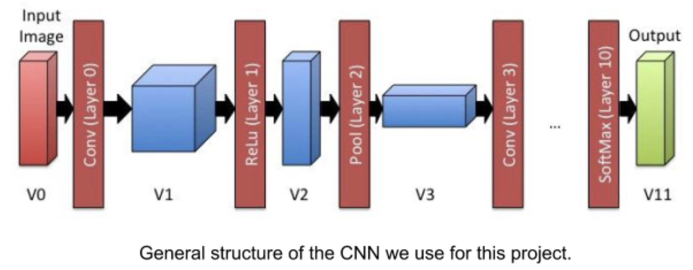
At a high level, a CNN consists of multiple layers. Each layer takes a multi-dimensional array of numbers as input and produces another multi-dimensional array of numbers as output (which then becomes the input of the next layer). When classifying images, the input to the first layer is the input image (e.g. 32x32x3 numbers for 32x32 pixel images with 3 color channels), while the output of the final layer is a set of likelihoods of the different categories (i.e., 1x1x10 numbers if there are 10 categories).
Each layer has a set of weights associated with it—these weights are what the CNN “learns” when it is presented with training data. Depending on the layer, the weights have different interpretations, but for the purpose of this project, it is sufficient to know that each layer takes the input, performs some operation on it that is dependent on the weights, and produces an output. This step is called the forward pass: we take an input and push it through the network, producing the desired result as an output. The forward pass is all that needs to be done to use an already-trained CNN to classify images.
In practice, a neural network really ends up being a pretty simple pattern recognition engine (with remarkably limited capacity), but it can be quite bizarre in what it ends up recognizing. For example, someone might train a neural network to recognize the difference between “dogs” and “wolves”. And it worked very well… by seeing the snow and the forest trees in the background of the wolf photos.
Your Task
There is much research done on different neural network architectures and training methods. However, another crucial aspect of neural nets is, given a trained network, actually classifying images in a fast and accurate way. That’s where your 61C knowledge comes in. For this project, you’re given a pre-trained network that can classify 32x32 RGB images into 10 categories. The images are taken from the CIFAR-10 dataset. The binary version (suitable for C programs) is already loaded onto Hive machines.
The network will already have the finalized weights, and the algorithm for computing the forward pass of the network is given to you. You’ll be speeding up the forward pass so that it can classify at a much quicker rate.
Step 1: Understanding the Code
Please read this section before trying to implement anything! There is quite a bit of code in this project, so it’s crucial that you have at least a high-level understanding of each file.
This project is also more open-ended than previous projects—you can speed up the application in any number of ways as long as it still produces the correct results. Don’t let this intimidate you! It is absolutely possible to get the required speedup without doing every possible optimization.
Directory Structure
When you pull the starter files from the GitHub classroom repository, your top-level directory structure should look like this:
Makefile
layers.h
snapshot/
layers_baseline.c
test/
benchmark.c
network.c
volume.c
network.h
volume.h
huge_test.sh
network_baseline.c
layers.c
run_test.sh
For this project, the only files you should change (and will submit) are:
layers.cnetwork.cvolume.c
This implies that while you are free to write your own helper methods in any of these files, their use will be restricted to that file since you will not be editing the .h files.
For convenience, we have provided the layers_baseline.c, network_baseline.c, and volume_baseline.c files. These _baseline.c files should not be modified when you’re writing your optimized code; they are there so that you can
- Measure your speedup and
- Reference a fully-correct (albeit slow) implementation.
Code Overview
There are a number of datatypes that are used in this project. By datatype, we mean structs that have been typedef‘d to have meaningful names. We highly encourage that you look around in the .h files to see what fields each datatype has. The header files are also where you’ll find a high-level description of what each function does. For the layers_baseline.c implementation, there are also comments with detailed explanations of what the code is doing.
The first datatype we’ll consider is the volume_t type, which contains a three-dimensional array (or Volume) of doubles. These are used to represent both the results of each layer, as well as the weights for some of the layers themselves.
Next, we have a number of different kinds of layers: conv, relu, pool, fc, and softmax. You do not need to understand what these different layers are doing, but each of them has:
- A data structure holding a description of the layer’s parameters. Note that each layer has a fixed set of parameters that don’t change during execution. They determine (for example) the size of its input and output volumes, and are set when the CNN is defined. For example, the CNN we are using has 3 conv layers, each with slightly different parameters.
- A
*_forwardfunction which performs the layer’s main operation. These functions first take the layer’s struct, as well as an array of pointers to input and output volumes. They also acceptstartandendindices into this array. This allows each layer to process a batch of inputs at once, which you may use for your optimizations. For example, you could have an array with pointers to input volumes and setstart = 5andend = 9to process inputs5,6,7,8,9at once and write the results into the corresponding entries of the output array. - Two functions,
make_*and*_load. The first generates a layer with a specific set of parameters, the second loads any weights for this layer from the file system.
The final important data structure is network_t, which holds all the information describing the CNN. This includes all layers, and an instance of each of the different intermediate Volumes. Note that these Volumes are not used for actually storing data (this is done by the batches we will describe below). They are there to make the dimensions of the different volumes easily available in one place.
All intermediate data is represented as batches. You can think of them as the intermediate data associated with a set of input images. While their type looks complicated (batch_t is shorthand for volume_t**), these are just two-dimensional arrays of pointers to Volumes. The first dimension tells you which layer the Volume belongs to (i.e., V0, V1, etc. in the figure above) and the second dimension tells you which input you are looking at. In the starter code we gave you, we only ever look at batches of size 1 (i.e., we process one sample at a time), but you may need to modify your program to consider larger batches, in order to parallelize computation. Batches can be allocated using the make_batch function and are freed with free_batch.
Finally, the net_forward function takes a batch (as well as start/end indices) and applies the CNN to each entry from start to end by calling the forward functions for each layer. This function is used in net_classify to take a set of input images, put them each into the V0 volume of a single-element batch, and then run the network on them. We save the likelihoods (i.e. the values in the last layer of the network) into a 2D matrix of doubles so that we can see how the network would classify the image. Be careful about these functions: they are called by the benchmarking code, so the function signature and its output should not be changed by your optimizations.
Conclusion
We recognize that this is a lot of information to digest, and that the above information is not sufficient to fully understand every detail of the code. Fortunately, you won’t need to do so in order to make it run faster: by looking at the structure of the code, you should be able to see potential sources of parallelism and other ways to optimize the code. Below, we will give you some first steps to get begin, and also provide you with a number of hints to try out. From there, you should experiment with different techniques and see how well they work.
Step 2: Profiling and Amdahl’s Law
Whenever you start optimizing some given code, you first have to determine where it spends most of its time. For example, speeding up a part of the program that only takes 5% of the overall runtime will at most get you 5% a speed-up and is probably not worth your time.
In lecture, you heard about Amdahl’s law, which is a great way to estimate the expected performance impact of an optimization. As we saw in class, to apply Amdahl’s law, we first have to find out what fraction of time is spent in the different parts of the program.
Using Gprof
Gprof is a tool that we will be using to profile the starter code to see which functions benefit the most from optimization. To run Gprof, we first need to compile the starter code with the “-pg” flag enabled:
$ make clean
$ make baseline CFLAGS="-Wall -Wno-unused-result -march=haswell -std=c99 -fopenmp -pg -O0"
Then, we need to run the starter code. Since Gprof is collecting statistics about the program, this will take a bit longer than usual (it took around 2 minutes for ours to finish). Make sure you execute this command on a hive machine.
$ ./benchmark_baseline benchmark
Finally, we need to see the results of Gprof.
$ gprof benchmark_baseline | less
The command we just ran should show a decent amount of text. For this project, we’re interested in the table at the top, with the following headers:
 %   cumulative   self              self     total
time   seconds   seconds    calls   s/call   s/call  name
The columns we are most interested in are:
% time: The amount of time we spend in a functioncalls: The number of times we call a functionname: The name of the function.
Interpreting Results
First, list the top 10 functions by how much percent of time our program spends in them. Amdahl’s law tells us which functions would benefit the most from optimization, so we recommend that you focus your time on these top 10 functions.
Note that some relatively simple functions may be in the top 10 because they are called many times (on the order of millions for some as compared to thousands for others). While optimizing these would certainly speed up our program, these functions may be so short that it’s difficult to optimize. Be aware of this should you try to optimize them.
Intermediate Profiling
If you ever want to profile your optimized code to see what you need to focus on, run the following commands:
$ make clean
$ make CFLAGS="-Wall -Wno-unused-result -march=haswell -std=c99 -fopenmp -pg -O0"
$ ./benchmark benchmark
$ gprof benchmark | less
These times will not be completely accurate since gprof does slow the execution down, but they will give you the general idea of what fraction of the time a function uses.
Step 3: Unrolling and Other Optimizations
In Step 2, we found the functions that are most worth optimizing. You should first try to speed up the computation by trying to apply conventional code optimizations (i.e. without SIMD or multiple threads). While we won’t tell you all the exact steps, here are some hints that should help you get started:
- Sometimes you can replace a function by multiple specialized functions that do the same thing but are optimized for specific input values. You would then call these specialized functions as applicable from the original function.
- Are there any places in the program where a variable always has the same value, but it is loaded from memory every time?
- Are there any places where you could do manual loop unrolling?
- Can you classify multiple samples at once instead of classifying them one after the other?
- Is there a better ordering of the different loops?
Note that the above hints relate to general optimization practices. You do not necessarily need to do all of these to achieve a good speedup.
Once you have improved performance using these optimizations, you can start applying vectorization and parallelization to make the program even faster. Note that you have considerable freedom to apply any of these optimizations, and there is more than one correct solution. Try to experiment with different approaches and see which one gives you the best performance.
Step 4: SIMD Instructions
In your lab, you learned how to apply SIMD instructions to improve performance. The processors in the hive machines support the Intel AVX extensions, which allow you to do SIMD operations on 256 bit values (not just 128 bit, as we have seen in the lab). You should use these extensions to perform four operations in parallel (since all floating point numbers are doubles, which are 64 bit in size).
As a reminder, you can use the Intel Intrinsics Guide as a reference to look up the relevant instructions. You will have to use the __m256d type to hold 4 doubles in a YMM register, and then use the _mm256_* intrinsics to operate on them.
Step 5: OpenMP
Finally you should use OpenMP to parallelize computation. Note that the easiest way to parallelize the classification of a large number of images is to classify batches of them in parallel (since these batches are independent). Note that you will need to make sure that none of the different threads overwrites each others’ data. Just adding a #pragma omp parallel for may cause errors.
Note that the hive machines have 4 cores with two hyperthreads each. This means that you should expect a speed-up of 4-8x (note that hyperthreads mean that two different programs execute on the same physical core at the same time; they will therefore compete for processor resources, and as a result, you will not get the same performance as if you were running on two completely separate cores).
Testing for Correctness
For this project, you will need to do your testing on the Hive machines so that your code has access to the dataset. There are three main techniques that we recommend you test your code. Before each of these, you must have compiled your code by running:
$ make clean && make
We run a make clean before running make to be absolutely sure that your files are being compiled for the Hive machines, and for grading we will use our own copy of the makefile.
Regular Benchmark
You can run
$ ./benchmark benchmark
To test how fast your code runs on a subset of 1200 images. The starter code takes around 13 seconds to finish running on the Hive machines. If you run this command with no extra arguments, you should see the following output:
RUNNING BENCHMARK ON 1200 PICTURES...
Making network...
Loading batches...
Loading input batch 0...
Running classification...
78.250000% accuracy
_________ microseconds
Your output will have a number that represents how long it takes for the network to classify. Note that we are only timing your network’s classification speed. The time it takes to load images into memory or other setup/teardown tasks are not included in the above execution time.
The accuracy line is a quick check to make sure that your implementation is correct; if the accuracy is any different (i.e. not 78.25%), that signifies that there is some issue with your implementation. For a more detailed look into what’s wrong with your code, run the run_test.sh or huge_test.sh scripts (described below) to narrow down the layers that might have a bug.
If this test takes too long, you can run the benchmark with a smaller number of images as follows:
$ ./benchmark benchmark n
Where n is an integer representing the number of images I want to run the benchmark on. Note that in this case, the accuracy may not be exactly 78.25% since we are testing on a different subset of images. To make sure your implementation is correct, you can run the following commands:
$ make baseline
$ ./benchmark_baseline benchmark n
Where the n is the same as above. Now, you can compare the accuracies outputted by these two commands and, if they are not the same, that means there’s definitely a bug in your implementation. However, even if they are the same, you should use the following two testing methods to fully verify the correctness of your implementation.
run_test.sh
This script runs your network on 20 images and outputs the exact values of each layer in the network. It compares them a set of reference values that were generated by the unoptimized starter code and checks if the values are the same (up to a reasonable degree of error to account for floating point errors).
It also runs your code on increasingly large subsets of images to catch any subtle parallelism bugs. For these parallel tests, we just compare the output of the last layer of your network with that of the unoptimized starter code.
This is a much more fine-grained test than just running ./benchmark benchmark since it makes sure that your network performs virtually the same computations as the starter code. We recommend that you run this after making any kind of major change to your code to make sure that the change did not impact your code’s correctness.
huge_test.sh
This script is almost the same as run_test.sh, except it also runs the code on two very large subsets of images. You likely won’t need to run this often (since it does take a decent amount of time to execute), but we recommend that you run this before submitting your project.
Debugging
As with previous C projects, we recommend you use CGDB and Valgrind to find bugs in your project. To use CGDB, we need to add the “-g” flag in our CFLAGS so that the debugging symbols are generated. We can accomplish this by executing:
$ make CFLAGS="-Wall -Wno-unused-result -march=haswell -std=c99 -fopenmp -g -O0"
$ cgdb ./benchmark
Then, in cgdb, you can set breakpoints and execute
run benchmark
to start debugging.
If you’re encountering a segfault in your code, Valgrind is great for narrowing down where the segfault is occurring. A sample command you might run is:
$ valgrind --leak-check=full --show-leak-kinds=all ./benchmark benchmark
Note that executing your program in valgrind will take much longer than usual.
Logistics
Please start early! Because there are many more 61C students than Hive machines, you will likely share resources with your classmates. This might affect the measurement of your code’s speedup. We encourage you to use Hivemind to help balance the load amongst the hive machines.
Measuring Your Speedup
To measure your speedup, you should run
$ make compare
and note the running time for your code (which is executed first) as compared to the benchmark (executed second).
Grading Rubric
In this project your grade will be determined based upon how fast your code runs relative to the naive solution given to you. Note that if your implementation does not pass run_test.sh, it will receive a score of 0 on the project. We will be using the following function to determine your grade:
grade(speedup):
    if 0 <= speedup < 1:
        0
    if 1 <= speedup <= 16:
        1 - (speedup - 16)^2 / 225
    if speedup > 16:
        1
For reference, here are the grades for some the speedup values:
| Speedup | Grade |
|---|---|
| 16x | 100% |
| 14x | ~98% |
| 12x | ~93% |
| 10x | ~84% |
| 8x | ~72% |
| 6x | ~56% |
| 4x | ~36% |
| 2x | ~13% |
Your speedup will be based off of how fast the code performs on our selected dataset, not necessarily just by running make compare. That being said, make compare is a good estimate for your performance as compared to the naive program that is given to you. We will test your program’s speed on the hive machines. You should test on the hive machines at a minimum to ensure everything is correct and working properly, but note that because of the size of the course the peak hours of the project right before it is due may not be an accurate reflection of your speedup if the hive machines get too busy. As a result, starting early is your friend and similarly your tests will likely be more accurate at 3am than noon.
We may also find it necessary to alter the exact means of determining your speedup. Currently the time to complete your program is measured by a Python script. If this proves to be too inconsistent, modifications may be made but they should not impact your results significantly. When testing your speedup also be sure to run the program a couple times and ensure that you can consistently achieve the speedup desired, as while we will average your speedup over multiple runs, the potential for complications is always present.
Submission
This project will have a submission on Gradescope, but because of the
hardware-specific nature of the project, the speedup comparison cannot be run
on Gradescope. You should submit to the assignment Project 4 - Submission,
which will check that your code compiles and that the accuracy has not changed.
The score on this assignment is irrelevant to your final grade, but any
submissions that do not compile or that affect the accuracy of the results will
not receive any credit.
Please submit the files layers.c, network.c, and volume.c to
Gradescope. Submit all three files since we will not be able to compile your
submission without all of them.
Over the course of the project, we will periodically pull the submissions from Gradescope and run them ourselves, updating the scores once we are finished. We will download the submissions to run tests at the following times:
- August 3rd at 10:00 AM Pacific
- August 5th at 10:00 AM Pacific
- August 8th at 10:00 AM Pacific
- August 9th at 10:00 AM Pacific
- August 10th at 10:00 AM Pacific
We may add additional dates to this list, but we will download submissions at these times at the minimum.
Once tests are completed, we will provide results to you on Gradescope and make a piazza announcement.
References
- Learning Multiple Layers of Features from Tiny Images, Alex Krizhevsky, 2009.
- Andrej Karpathy’s ConvNetJS implementation. https://cs.stanford.edu/people/karpathy/convnetjs/
- Gerald Friedland, An Explainable Neural Network. http://tfmeter.icsi.berkeley.edu