Instructions
Phase II
In this phase, we wish to see the effect of scheduling policies on the throughput under different transport protocols.
- Consider the following network topology.
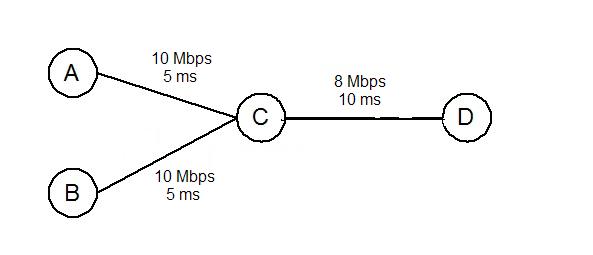
There is a CBR (Constant
Bit Rate) connection (which uses UDP) from node A to node D sending at a rate
of 3 Mbps. (You may want to set random_
to 1 to get rid of synchronization.) There is another connection from node B to
node D which generates Exponential On/Off traffic (Please refer to part
on Traffic generators in the NS Documentation) over UDP, with an
average burst time of 500 ms and average idle time of 500ms with the burst
rate equal to 6 Mbps. Assume that all packets are 1000 bytes in length.
Provide the graphs for the throughput for both the connections as a function of time for the following two cases.
- FCFS scheduler at node C. Assume that link C-D has a drop-tail queue of length = 40.
- Round Robin Scheduler at node C. Implement the two connections as belonging to different traffic classes (This sample code should be helpful). Also, assume drop-tail queues for each class of length = 20 (each).
For each of the parts above, answer the following question:
- Are the throughputs for the two connections fair? Why or why not? Please provide a clear reason. You may attach relevant plots to support your argument.
- We now
consider the topology shown below.
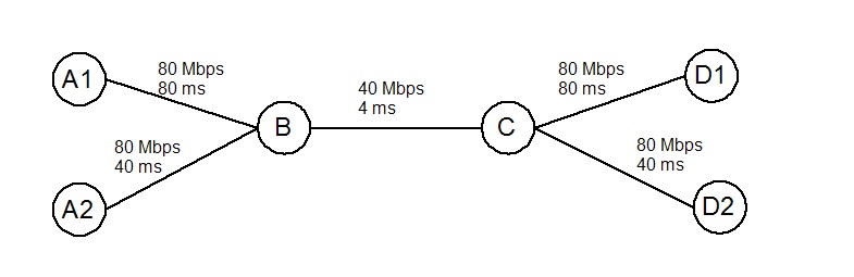
There is an FTP/TCP (TCP Reno) flow from A1 to D1 and another from A2 to D2. Note that the propagation delay from A1 to D1 is twice as large as the propagation delay from A2 to D2. Assume that each packet is 1250 bytes in length. This is the same question as the part 2 in phase 1. The difference in this case is we wish to implement a Round Robin Scheduler at B. Assume that the queue for each class at B can hold upto 130 packets. Run the simulation for 1500 seconds. - Please provide a graph of the window size as a function of time.
- Also, provide a graph of the throughput obtained as a function of time.
Now answer the following questions:
· How does the round-robin scheduling compare to the case of FCFS scheduling at node B?
· Does it lead to equal rates (fairness) for the two flows in spite of a difference in RTTs?
· If it is fair, why is it so? If not, why not?
Tips
- Avoid using the trace-all/namtrace-all feature for long simulations -- it will fill up your disk quota.
- For all simulations, set window_ variable for all TCP agents to 100000 to ensure that the receiver window size does not become a bottleneck.
- Sections on “Queue Management and Packet Scheduling” and “Traffic Generators” in the NS Documentation should be useful for this project.
Project Submission
Phase II
Submit a report along with the ns-2 scripts used together in a single tar file. Email the tar file to ee122-ta@imail.eecs.berkeley.edu, ee122-tb@imail.eecs.berkeley.edu with the subject line as "EE122 Project Phase II" by 11.59 pm, April 11, 2006.
Resources
- ns-2 is installed on the instructional machines under /share/instsww/pkg/ns-allinone-2.27-fasttcp. To run it from your account make sure to add /share/instsww/ns-allinone-2.27-fasttcp/bin to the PATH environment variable and /usr/sww/lib to the LD_LIBRARY_PATH variable.
- ns-2 online documentation is here.
- gnuplot is a good tool for generating plots. You will find useful links here.