Nomenclature
Feasible set
What is a solution? Optimal value, optimal set
Local vs. global optima
Consider the optimization problem

Feasible set
The feasible set of problem  is defined as

A point  is said to be feasible for problem if it belongs to the feasible set
  , that is, it satisfies the constraints.
Example: In the toy optimization problem, the feasible set is the ‘‘box’’ in  , described by
  ,
,  .
.
The feasible set may be empty, if the constraints cannot be satisfied simultaneously. In this case the problem is said to be infeasible.
What is a solution?
In an optimization problem, we are usually interested in computing the optimal value of the objective function, and also often a minimizer, which is a vector which achieves that value, if any.
Feasibility problems
Sometimes an objective function is not provided. This means that we are just interested in finding a feasible point, or determine that the problem is infeasible. By convention, we set  to be a constant in that case, to reflect the fact that we are indifferent to the choice of a point as long as it is feasible.
Optimal value
The optimal value of the problem is the value of the objective at optimum, and we denote it by  :
:

Example: In the toy optimization problem, the optimal value is  .
.
Optimal set
The optimal set (or, set of solutions) of problem is defined as the set of feasible points for which the objective function achieves the optimal value:

We take the convention that the optimal set is empty if the problem is not feasible.
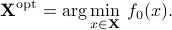
A standard notation for the optimal set is via the  notation:
A point is said to be optimal if it belongs to the optimal set. Optimal points may not exist, and the optimal set may be empty. This can be due to the fact that the problem is infeasible. Or, it may be due to the fact that the optimal value is only attained in the limit.
Example: The problem

has no optimal points, as the optimal value  is only attained in the limit
  .
.
If the optimal set is not empty, we say that the problem is attained.
Suboptimality
The  -suboptimal set is defined as

(With our notation,  .) Any point in the -suboptimal set is termed -suboptimal.
This set allows to characterize points which are close to being optimal (when is small). Usually practical algorithms are only able to compute suboptimal solutions, and never reach true optimality.
Example: Nomenclature of the two-dimensional toy problem.
Local vs. global optimal points
A point  is locally optimal if there is a value
  such that is optimal for problem

In other words, a local minimizer minimizes , but only for nearby points on the feasible set. So the value of the objective function is not necessarily the optimal value of the problem.
The term globally optimal (or, optimal for short) is used to distinguish points in the optimal set from local minima.
Example: a function with local minima.
Local optima may be described as the curse of general optimization, as most algorithms tend to be trapped in local minima if they exist.