Solving linear equations via the QR decomposition
Basic idea
The QR decomposition of a matrix
Solution via full QR decomposition
Set of solutions
Basic idea: reduction to triangular systems of equations
Consider the problem of solving a system of linear equations  , where
  and
and  are given.
The basic idea in the solution algorithm starts with the observation that in the special case when  is upper triangular, that is,
  if
if  , then the system can be easily solved by a process known as backward substitution. In backward substitution we simply start solving the system by eliminating the last variable first, then proceed to solve backwards. The process is illustrated in this example, and described in generality here.
The QR decomposition of a matrix
The QR decomposition allows to express any  matrix as the product
  where
where  is
is  and orthogonal (that is,
  ) and
) and  is upper triangular. For more details on this, see here.
Once the QR factorization of is obtained, we can solve the system by first pre-multiplying with both sides of the equation:
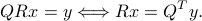
This is due to the fact that . The new system  is triangular and can be solved by backwards substitution. For example, if is full column rank, then is invertible, so that the solution is unique, and given by
 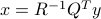 .
.
Let us detail the process now.
Using the full QR decomposition
We start with the full QR decomposition of A with column permutations:
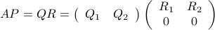
where
![Q = [Q_1,Q_2]](eqs/5486717721084986714-130.png) is and orthogonal ();
is and orthogonal (); is
is  , with orthonormal columns (
 );
);  is
is  , with orthonormal columns (
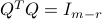 );
);  is the rank of ;
  is
is  upper triangular, and invertible;
 is a
is a  matrix;
 is a permutation matrix (thus,
  ).
). The zero submatrices in the bottom (block) row of
have  rows.
rows.
Using  , we can write
  , where
  . Let's look at the equation in
  in expanded form:
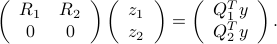
We see that unless  , there is no solution. Let us assume that . We have then
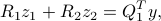
which is a set of linear equations in  variables.
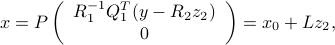
A particular solution is obtained upon setting  , which leads to a triangular system in
  , with an invertible triangular matrix . Hence
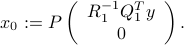
 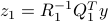 , which corresponds to a particular solution
  to
to  :
:
Set of solutions
We can also generate all the solutions, by noting that  is a free variable. We have
where
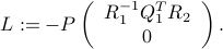
The set of solutions is the affine set 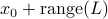 .
.