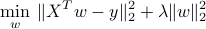
Kernel Least-Squares
Motivations
The kernel trick
Nonlinear case
Examples of kernels
Kernels in practice
Motivations
Consider a linear auto-regressive model for time-series, where  is a linear function of

This writes  , with
  the ‘‘feature vectors’’

We can fit this model based on historical data via least-squares:
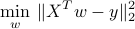
The associated prediction rule is  .
.
We can introduce a non-linear version, where is a quadratic function of

This writes 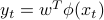 , with
  the augmented feature vectors

Everything the same as before, with  replaced by
  .
.
It appears that the size of the least-squares problem grows quickly with the degree of the feature vectors. How do we do it in a computationally efficient manner?
The kernel trick
We exploit a simple fact: in the least-squares problem
the optimal  lies in the span of the data points
  :
:

for some vector  . Indeed, from the fundamental theorem of linear algebra, every
  can be written as the sum of two orthogonal vectors:

where  (that is,
  is in the nullspace
  ).
).
Hence the least-squares problem depends only on  :
:
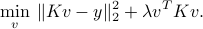
The prediction rule depends on the scalar products between new point and the data points  :
:

Once  is formed (this takes
  ), then the training problem has only
  variables. When
  , this leads to a dramatic reduction in problem size.
Nonlinear case
In the nonlinear case, we simply replace the feature vectors  by some ‘‘augmented’’ feature vectors
  , with
  a non-linear mapping.
This leads to the modified kernel matrix

The kernel function associated with mapping is
It provides information about the metric in the feature space, eg:

The computational effort involved in
solving the training problem;
making a prediction,
depends only on our ability to quickly evaluate such scalar products. We can't choose  arbitrarily; it has to satisfy the above for some .
Examples of kernels
A variety of kernels are available. Some are adapted to the structure of data, for example text or images. Here are a few popular choices.
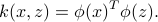
Polynomial kernels
Regression with quadratic functions involves feature vectors

In fact, given two vectors  , we have
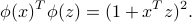
More generally when is the vector formed with all the products between the components of  , up to degree
  , then for any two vectors
  ,
,
The computational effort grows linearly in  .
.
This represents a dramatic reduction in speed over the ‘‘brute force’’ approach:
Form
,  ;
;evaluate
 .
In the above approach the computational effort grows as
.
In the above approach the computational effort grows as  .
.
Gaussian kernels
Gaussian kernel function:
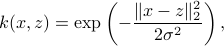
where  is a scale parameter. This allows to ignore points that are too far apart. Conrresponds to a non-linear mapping to infinite-dimensional feature space.
Other kernels
There is a large variety (a zoo?) of other kernels, some adapted to structure of data (text, images, etc).
Kernels in practice
Kernels need to be chosen by the user.
Choice not always obvious; Gaussian or polynomial kernels are popular.
We control over-fitting via cross validation (to choose, say, the scale parameter of Gaussian kernel, or degree of polynomial kernel).