Ordinary Least-Squares Problem
Definition
Interpretations
Solution via QR decomposition (full rank case)
Optimal solution (general case)
Definition
The Ordinary Least-Squares (OLS, or LS) problem is defined as
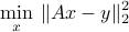
where  ,
,  are given. Together, the pair
  is referred to as the problem data. The vector
  is often referred to as ‘‘measurement‘‘ or “output” vector, and the data matrix
  as the ‘‘design‘‘ or ‘‘input‘‘ matrix.
The vector
as the ‘‘design‘‘ or ‘‘input‘‘ matrix.
The vector  is referred to as the residual error vector.
Note that the problem is equivalent to one where the norm is not squared. Taking the squares is done for convenience of the solution.
Interpretations
Interpretation as projection on the range
 |
We can interpret the problem in terms of the columns of 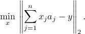
In this sense, we are trying to find the best approximation of As seen in the picture, at optimum the residual vector |
![A = [a_1, ldots, a_n]](eqs/7871202357948208737-130.png) , where
, where  is the
  -th column of
  . The problem reads
 's (that is to say: the range of
 Examples:
Interpretation as minimum distance to feasibility
The OLS problem is usually applied to problems where the linear  is not feasible, that is, there is no solution to .
The OLS can be interpreted as finding the smallest (in Euclidean norm sense) perturbation of the right-hand side,  , such that the linear equation

becomes feasible. In this sense, the OLS formulation implicitly assumes that the data matrix of the problem is known exactly, while only the right-hand side is subject to perturbation, or measurement errors. A more elaborate model, total least-squares, takes into account errors in both and .
Interpretation as regression
We can also interpret the problem in terms of the rows of , as follows.
Assume that ![A^T = [a_1, ldots, a_m]](eqs/4224999647760616708-130.png) , where
, where  is the
  -th row of ,
  . The problem reads
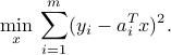
In this sense, we are trying to fit of each component of as a linear combination of the corresponding input  , with
  as the coefficients of this linear combination.
Examples:
Solution via QR decomposition (full rank case)
Assume that the matrix  is tall (
 ) and full column rank. Then the solution to the problem is unique, and given by
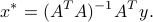
This can be seen by simply taking the gradient (vector of derivatives) of the objective function, which leads to the optimality condition 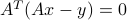 . Geometrically, the residual vector
  is orthogonal to the span of the columns of , as seen in the picture above.
We can also prove this via the QR decomposition of the matrix :  with
with  a
a  matrix with orthonormal columns (
 ) and
) and  a
a  upper-triangular, invertible matrix. Noting that

and exploiting the fact that is invertible, we obtain the optimal solution 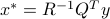 . This is the same as the formula above, since

Thus, to find the solution based on the QR decomposition, we just need to implement two steps:
Rotate the output vector: set
 .
.Solve the triangular system
 by backwards substitution.
In Matlab, the backslash operator finds the (unique) solution when is full column rank.
>> x = A\y;
Optimal solution and optimal set
Recall that the optimal set of an minimization problem is its set of minimizers. For least-squares problems, the optimal set is an affine set, which reduces to a singleton when is full column rank.
In the general case ( not necessarily tall, and /or not full rank) then the solution may not be unique. If  is a particular solution, then
  is also a solution, if
  is such that
  , that is,
  . That is, the nullspace of describes the ambiguity of solutions. In mathematical terms:
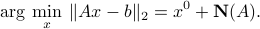
The formal expression for the set of minimizers to the least-squares problem can be found again via the QR decomposition. This is shown here.