Name 1:
Login: ee16a-
Name 2:
Login: ee16a-
Table of Contents
- Checkoff Outline
- Setup
- Images and Data Grids
- Real Image Scanning
Overview
This week, you will scan an image pixel by pixel and write code to recreate it with the sensor readings. Specifically, you will begin by checking that the circuit you built last time still works and that the projector is correctly connected to the computer. Next you will write code to generate the pattern that the projector will use to scan through the image. Finally you will use your code and scanning matrix to image a card!
Task 1a: Light Sensor
Set the solar cell up with your low pass filter circuit as you had in week I.
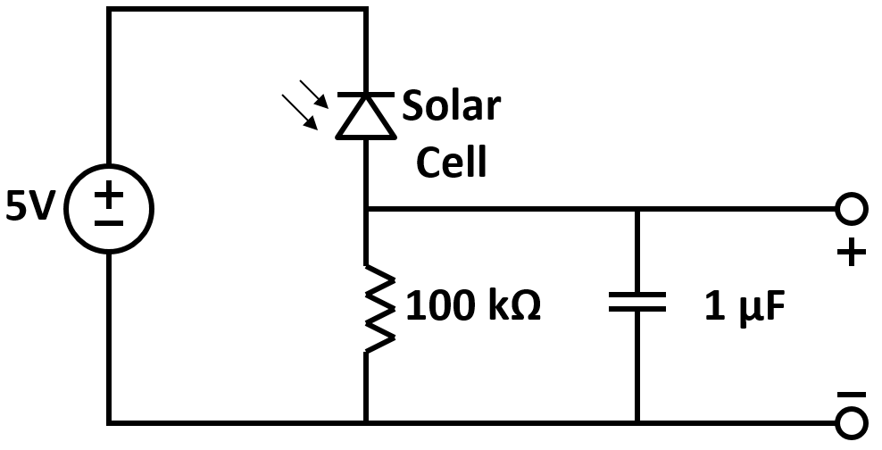
Use the oscilloscope to confirm that the sensor you built last week still responds to changes in light. You should be able to reproduce the same output you saw before.
Task 1b: Upload Arduino Code
We will be using a different Arduino program this week.
Upload the AnalogReadSerial program to your Arduino.
Task 1c: Projector Setup
- Place the breadboard, Arduino, and solar cell in the stand.
- Connect the USB cable to the Arduino.
- Connect the HDMI and power cables to the projector.
- Turn on the projector and select the HDMI output.
Confirm that you are able to see a blank Windows Desktop on the projector screen.
#Import Necessary Libraries
from  pylab import *
import struct
import numpy
import time
import scipy
from scipy import linalg
import serial
Task 2a: Working with Images
In order to create the pattern of the white pixels illuminating, we will use data-grids. A simple black-and-white image can be represented using a 2D data-grid, where the value in each cell represents the grayscale value in the image.
To see how this works, create a 5x5 data-grid with random values between 0 and 1 and print the data-grid. You might find np.random.random helpful.
Create a random 5x5 matrix
# TODO: Make a random data-grid
# random_image =
Display the same matrix with plt.imshow.
plt.imshow(random_image, cmap='gray', interpolation='nearest')
What do you notice about the relationship between how numbers between 0 to 1 relate to grayscale colors? What color would 1 correspond to? What about 0?
Task 2b: Scanning Matrix
Next, we will create a matrix that we can use to illuminate individual pixels for our single pixel camera. The first step is to think about the image as a vector (you will see why this is important soon).
**
Say we look at the same random_image that you created. Convert the matrix to a vector and display it. You will find the command np.reshape helpful. What do you notice? **
##TODO: Convert matrix to vector
#random_image_vector =

##Display the vector
plt.imshow(random_image_vector, cmap='gray', interpolation='nearest')
plt.savefig("random_image_vector.png")
Imaging Mask
Ok, but what is the point of all this? Given a vector of sensor readings from our single pixel camera, we want to be able to recreate the image with the help of a few mathematical operations.
Let's begin by creating a fake vector of sensor readings - essentially the same vector as random_image_vector. Except we will not simply use that vector. We will use matrix multiplication!
What matrix, multiplied with random_image_vector should return random_image_vector? Your answer should be a fairly simple matrix, which we will call the imaging mask ($H$).
This operation is represented in the following equation:
where $H$ is the imaging mask, $i$ is the image vector and $s$ is the sensor reading vector.
** Create the imaging mask $H$. What dimensions does it have and why? **
##TODO: Create the multiplication matrix
#H =

#Display this image mask
plt.imshow(H, cmap='gray', interpolation='nearest')
**
Now multiply this matrix with random_image_vector to get the same vector back!**
##TODO: Recreate the random_image_vector by multiplying the two matrices
#random_image_recreate =

##Display the result and compare to random_image_vector
plt.imshow(random_image_recreate, cmap='gray', interpolation='nearest')
What is happening in this matrix multiplication? Each column of vector H is responsible for "illuminating" a single pixel in the random image!
Think about the vector random_image_vector. We created it by converting the 5x5 image into a vector. Similarly, every column in the matrix H can be represented as the vector version of a simple 5x5 image.
** To see this, iterate through each column of matrix H, convert it to a 5x5 image, and check that it is actually illuminating each pixel of the 5x5 image!**
##TODO: Iterate through columns of matrix H and form individual masks
figure(figsize=(20,20))
for j in range(0,25):
    subplot(5,5,j+1)
    #proj = (reshape command!)
    imshow(proj,cmap='gray', interpolation='nearest');
    title('Mask ' + str(j))
Now let's try an imaging mask that's a bit more complicated. Say we want our fake sensor reading vector to have the sensor values for every other pixel (1,3,...), then the pixels we skipped (2,4,...).
** Repeat the above procedure with a new imaging mask, $H1$ that selects alternate pixels. **
##TODO: Create the multiplication matrix


#Display this image mask
figure()
plt.imshow(H1, cmap='gray', interpolation='nearest')

##TODO: Recreate the random_image_vector by multiplying the two matrices
#random_image_recreate1 =

#Display the result and compare to random_image_vector
figure()
plt.imshow(random_image_recreate1, cmap='gray', interpolation='nearest')
Task 3: Imaging Real Pictures
Finally, we will use our two matrices to image a real picture. Because our picture is fairly large, we want each individual mask to have dimensions 40x30 to match the 4:3 aspect ratio of the projector. To do so, ** recreate your masks $H$ and $H1$ to match these dimensions of an individual mask. **
##TODO: Recreate H

##TODO: Recreate H1
In order to tell the imaging code to use a specific matrix, we save it into a variable called imaging_mask.
np.save('imaging_mask.npy', H)
From the command line (in the current directory), run
python capture_image.py
The script projects patterns based on the masks you designed, imaging_mask.npy. The sensor readings will then be saved into an array named sensor_readings.npy.
After the sensor readings have been captured, load the sensor reading vector. Here is the equation relating H, sensor readings, and image vector:
$$H * i = s$$** Recreate the image vector from the sensor readings. **
sr = np.load('sensor_readings.npy')

#TODO: Create the image vector from H and sr
#iv =

#Display the result
plt.figure(figsize=(3,4))
plt.imshow(np.reshape(iv,(30,40)), cmap='gray', interpolation='nearest')
Congratulations! You have imaged your first image using your single pixel camera! Does your recreated image match the real image? What are some problems you notice?
Here are some example images that we recreated using this setup:


** Next, use the second mask for imaging. Can you repeat the same procedure by just replacing $H$ with $H1$? Why or why not?**
np.save('imaging_mask.npy', H1)
Now run capture_image.py from the command line again (make sure to restart the script) to collect sensor readings, then reconstruct the image.
sr = np.load('sensor_readings.npy')

#TODO: Create the image vector from H and sr
#iv =

#Display the result
plt.figure(figsize=(3,4))
plt.imshow(np.reshape(iv,(30,40)), cmap='gray', interpolation='nearest')
You are done for the week! Save your code and low pass filter circuit for next week, where you will illuminate multiple pixels per mask!