Name 1:
Login: ee16a-
Name 2:
Login: ee16a-
Introduction
There are various positioning systems in our life, and we use them everyday. The most commonly used one is the Global Positioning System (GPS). The navigation systems in the cars, the Google Map, cell phones, and even rockets and spaceships all use the GPS.
In this lab, we are going to explore the basics of these navigation systems and build our own. At the end of this lab, you will be able to determine your location in a 2D area using just a microphone!
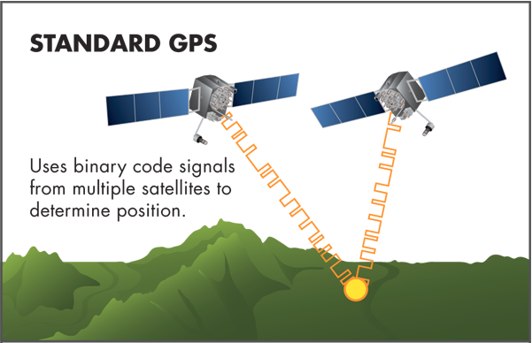
Basic Principle of Operation
GPS satellites broadcast a variety of measurements including time from a very precise clock, as well as the satellite's position, velocity, etc. GPS receivers make use of the fact that light propagates at a known speed, so the receiver can compute distance from the satellite by measuring how long it takes the GPS signal to propagate from the satellite to the receiver.
 **Source**: [Kathleen Cantner, AGI](http://www.earthmagazine.org/article/precise-fault-how-gps-revolutionized-seismic-research)
Just like the GPS, we will use speakers as our signal emitters (like the "GPS satellite"), and use microphones (our version of the "GPS chip") to receive the signals. Based on the delay between the times at which we receive each signal we can determine distances.
%pylab inline
import numpy
%run wk1_code/virtual.py
%run wk1_code/signals.py
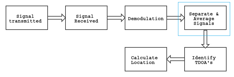
Extracting Information
The block diagram the below shows a high level overview of the full system. We begin by transmitting the signal from the speakers. This signal is then recorded by the microphone and converted to a format we can use for further processing. Next the signals from each speaker are identified and the time differences are used to determine locations.
Task 1: Measuring the Similarity of Two Signals
Just like real GPS, our system will have multiple speakers emitting signals, but only a single microphone receiving them. The signal that we receive from the microphone will therefore be a sum of the individual speaker outputs. In order to determine which signal came from which speaker, we must first separate our raw received signal back into the components that correspond to each speaker. In order to identify the different components in our single recorded microphone signal we will use a tool called cross-correlation.
Cross-correlation is a measure of similarity between two signals calculated by taking successive products as one function slides past the other. More intuitively this is a measure of the "common area" or "overlap" between two signals with respect to time. For discrete signals, the "common area" at time $t$ is the product of the two signals evaluated at that time. Both a mathematical definition and an animation are shown below:
$$(f \star g)[n]\ \stackrel{\mathrm{def}}{=} \sum_{m=-\infty}^{\infty} f^*[m]\ g[m+n]$$
Note: This definition is for general complex valued functions; for purely real valued signals we can ignore the $f^*[m]$ denoting the conjugate of $f$ and see that this is indeed a sum of shifted products.

Each of our signals is a sequence of scalar values. Is there a concept we have already covered in this course that could be used to represent this?
The value of the cross-correlation at each time step is the sum of the products of overlapping samples from each signal. Our mathematical definition above shows a sum from $-\infty$ to $\infty$, however in this lab we know our signals only have a finite number of values define the value at all other times to be 0; because of this we only need to compute the cross-correlation for the times at which the signals overlap (all other values will be 0).
As a simple, concrete example let's define signal $x_1=[1,2,3]$ and $x_2=[3,2,1]$. In order to change the size of these signals we can either append or prepend zeros. To compute the first sample of cross-correlation, we will shift $x_2$ left until the last value of $x_2$ overlaps with the first sample of $x_1$. We now compute the product of the overlapping values: $1\times 1= 1$. To calculate the second value of the cross-correlation we shift $x_2$ to the right and sum the products: $(2\times 1)+(1\times 2) = 2 + 2 = 4$. We continue this process until the last sample of $x_1$ overlaps with the first value of $x_2$.
Each value of the cross-correlation is a sum of products between individual elements from our sequences of values. Is this an operation we have already used in this class?
# Input signals for which to compute the cross-correlation
signal1 = np.array([0, 1, 2, 3, 3, 2, 1, 0])
signal2 = np.array([1, 2, 3, 1, 1])
print np.correlate(signal1, signal2, 'full')

# Pad with zeros to make the signals an appropriate size.
# How should we choose this size?
signal1 = np.lib.pad(signal1, (0, 4), 'constant')
signal2 = np.lib.pad(signal2, (0, 2*(4)-1), 'constant')

# Circularly shift signal2 until the last sample of signal 2 is aligned with the first sample of signal1
# Using a circular shift with the numpy.roll function is a convenient way to simulate shifting signals over time
signal2 = np.roll(signal2, -(5-1))

# Although we are circularly shifting, it makes more sense to plot it in terms of negative values
signal2_plot = np.roll(signal2, -1)

# Plot each operation required to compute the cross-correlation
plt.figure(figsize=(12,14))
for i in range(3*4):
    plt.subplot(4,3,i+1)
    plt.stem(signal1, 'b--', label='Signal 1')
    plt.stem(range(-len(signal2_plot)+1+i,i+1), signal2_plot, 'g-', label='Signal 2')
    plt.xlim(-12, 12)
    plt.ylim(0, 4)
    plt.title('cross-correlation(%d)=%d\n%s\n%s'%(i, np.dot(signal1, signal2), str(signal1), str(signal2)))
    signal2 = np.roll(signal2, 1)

# Adjust subplot spacing
plt.tight_layout()

Based on example shown above, implement the function below that will compute and return the cross-correlation of two input signals.
Things to consider:
- Built in
numpyfunctions to compute sums of products mentioned above - Lengths of the input signals
- Length of the output
- Built in
numpyfunctions shown above to append or prepend zeros to a signal
Hint: Python list operations tend to be slower thannumpyarray operations for long signals (in particular appending python lists together). When computing the cross correlation try defining a numpy array of zeros of the known output length and setting individual values of it. An example is shown in the skeleton code below.
def cross_correlation(signal1, signal2):
    """Compute the cross_correlation of two given signals
    Args:
    signal1 (np.array): input signal 1
    signal2 (np.array): input signal 2

    Returns:
    cross_correlation (np.array): cross-correlation of signal1 and signal2

    >>> cross_correlation([0, 1, 2, 3, 3, 2, 1, 0], [0, 2, 3, 0])
    [0, 0, 3, 8, 13, 15, 12, 7, 2, 0, 0]
    >>> cross_correlation([0, 2, 3, 0], [0, 1, 2, 3, 3, 2, 1, 0])
    [0, 0, 2, 7, 12, 15, 13, 8, 3, 0, 0]
    """
    # YOUR CODE HERE #

    # How long should the output be?
    output_length = len(signal1)

    # Example of using a numpy array for output rather than python list operations
    # Define an output array of fixed length
    output = np.zeros(output_length)

    # Compute and set each value of the output. The example returns an array of all ones.
    for i in range(output_length):
        output[i] += 1

    return output
You can compare your result to the correct one here:
def test_correlation_plot(signal1, signal2, lib_result, your_result):
    # Plot the output
    plt.figure(figsize=(16,4))
    plt.plot(range(len(lib_result)), lib_result, label='Correct Answer')
    plt.plot(range(len(your_result)), your_result, label='Your Answer')
    plt.legend()
    plt.title("Cross correlation of:\n%s\n%s"%(str(signal1), str(signal2)))
# You can change these signals to get more test cases
# Test 1
signal1 = np.array([1, 5, 8, 6, 4, 9, 2, 1, 1])
signal2 = np.array([1, 3, 5, 2])

# Run the test
lib_result, your_result = test_correlation(cross_correlation, signal1, signal2)
test_correlation_plot(signal1, signal2, lib_result, your_result)

# Test 2
signal1 = np.array([1, 3, 5, 2])
signal2 = np.array([1, 5, 8, 6, 4, 9, 2, 1, 1])

# Run the test
lib_result, your_result = test_correlation(cross_correlation, signal1, signal2)
test_correlation_plot(signal1, signal2, lib_result, your_result)

# Test 3
signal1 = np.array([1, 3, 5, 2])
signal2 = np.array([1, 5, 8, 6])

# Run the test
lib_result, your_result = test_correlation(cross_correlation, signal1, signal2)
test_correlation_plot(signal1, signal2, lib_result, your_result)
Task 2: Extracting Information
We now have a powerful tool to measure how similar two signals are, and will now explore how to use that in the context of our locationing system. Our locationing system will be transmitting what we will call a beacon signal from each speaker. In order to successfully identify the beacon signals with our single microphone recording, we would like for the same signal to have a large cross-correlation with itself, but a very small cross-correlation with all of the others.
Real GPS deals with this exact same problem and uses a solution called Gold Code. Gold codes are binary sequences (signals composed of just 1's and 0's) constructed with exactly this property: they have small mutual cross-correlation, but large cross-correlation with themselves. Gold codes are generated by performing the XOR logic operation between the beacon signal and a pseudo-random bit sequence as shown below. The theory and implmentation of Gold codes is beyond the scope of this class, but simply understanding the properties of cross correlation explained above is enough to show why we will be using them.

# Model the sending of precomputed beacons in Gold code
sent_0 = beacon[0][:1000]
sent_1 = beacon[1][:1000]
sent_2 = beacon[2][:1000]

# Model our received signal as the sum of each beacon
received = sent_0 + sent_1 + sent_2

# Plot the received signal
plt.figure(figsize=(16,2))
plt.plot(received)
plt.title('Received Signal (sum of beacons)')

print len(numpy.convolve(received, sent_1[::-1]))

# Plot the correlation of the received signal and a beacon
plt.figure(figsize=(16,6))
plt.subplot(2,2,1)
plt.plot(np.roll(cross_correlation(received, sent_1), 0))
plt.plot(numpy.convolve(received, sent_1[::-1]))
plt.title('Cross-correlation of received signal and and beacon 1')

# Plot the correlation of two beacons with each other
plt.subplot(2,2,2)
plt.plot(np.roll(cross_correlation(sent_0, sent_1), 0))
plt.plot(numpy.convolve(sent_0, sent_1[::-1]))
plt.title('Cross-correlation of beacon 1 and beacon 2')
plt.ylim(-500, 1500)
We can see that there is a peak around the 1000th sample in the second plot. We can conclude that the second beacon arrives at around $t=1000$ (Warning: the unit here is samples, not seconds!). We can also see that in the third graph, which is the cross-correlation of two signals in a Gold Code, there is no such a peak.
If you are given some beacon signals and a received signals, can you compute when (in sample) does each beacon signal arrive?
Implement a helper function identify_peak which takes in a signal with a single global maximum and returns the index of the peak of the signal.
def identify_peak(signal):
    """Returns the index of the peak of the given signal.
    Args:
    signal (np.array): input signal

    Returns:
    index (int): index of the peak

    >>> identify_peak([1, 2, 5, 7, 12, 4, 1, 0])
    4
    >>> identify_peak([1, 2, 2, 199, 23, 1])
    3
    """
    # YOUR CODE HERE #
    return 0
Implement a function arrival_time, which uses cross-correlation to identify the times at which each beacon arrived.
def arrival_time(beacons, signal):
    """Returns a list of arrival times (in samples) of each beacon signal.
    Args:
    beacons (list): list in which each element is a numpy array representing one of the beacon signals
    signal (np.array): input signal, for example the values recorded by the microphone

    Returns:
    arrival_time (list): arrival time of the beacons in the order that they appear in the input
    (e.g. [arrival of beacons[0], arrival of beacons[1]...])
    """
    # YOUR CODE HERE #
    return [0 for b in beacons]
Verify the following tests for each of the above functions passes.
test(cross_correlation, identify_peak, arrival_time, 2)
# If you didn't implment cross-correlation using numpy functions this may take a few minutes to run.
# If you used numpy functions to implement cross-correlation as suggested it should take < 10 sec
# For a length 10,000 signal how total operations would computing the cross-correlation take?
test(cross_correlation, identify_peak, arrival_time, 3)
Task 3: Separating Real Signals
Now that we have reviewed the theoretical basis of cross-correlation and shown that it can be used to separate simulated signals, we will test the same functions you wrote with real data.
Connect your microphone and speaker to the appropriate ports on the front of the computer.
First, we need to choose the input device we are using. Run the following code to select audio (input/output) devices:
%run wk1_code/rec.py
Now run the code below to define our API for recording signals:
def record_signal():
    """Get the signal from the microphone"""
    return mic.new_data()
Finally, we are ready to record the signal and test our functions! Play offset250_540-321.wav in the lab folder and use your microphone to record it (by running the cell below - you may want to run it for several times when the wav file is playing to clear the buffer.
received_signal = record_signal()
We can now plot the received signal - make sure the signal fills up the whole recording duration!
# Plot the received signal
plt.figure(figsize=(16,4))
plt.plot(received_signal)
Now you can test your code! Don't worry if you cannot understand the codes below - you will eventually understand that by the end of Lab 3!
# Convert the received signals into the format our functions expect
# If your arrival_times test ran slowly expect this code to run slowly as well
# If it takes more than a few minutes to run try taking only 5,000 samples of demod

%run wk1_code/demod.py
demod = demodulate_signal(received_signal)


sig = [cross_correlation(demod, b) for b in beacon[:4]]
sig = [average_signal(s) for s in sig]
# Plot the cross-correlation with each beacon
plt.figure(figsize=(16,4))
for i in range(len(sig)):
    plt.plot(range(len(sig[i])), sig[i], label="Beacon %d"%(i+1))
plt.legend()

# Scale the x axis to show +/- 1000 samples around the peaks of the cross correlation
peak_times = ([argmax(sig[i]) for i in range(len(sig))])
plt.xlim(max(min(peak_times)-1000, 0), max(peak_times)+1000)
As you can see (if you have the correct implementation), we have several nice peaks after doing the cross-correlation. Next week, we will use the information we have in this week (several arrival time in samples) to determine distances.
Copy cross_correlation, identify_peak, and arrival_time into a new text file called lab1.py.
You will need to use these functions for next week's lab!