Conic Duality
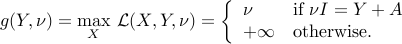
Conic problem and its dual
Strong duality and KKT conditions
SDP duality
SOCP duality
Examples
Conic problem and its dual
The conic optimization problem in standard equality form is:
where  is a proper cone, for example a direct product of cones that are one of the three types: positive orthant, second-order cone, or semidefinite cone. Let
  be the cone dual , which we define as
(
be the cone dual , which we define as
(
{cal K}^ast :={ lambda : forall : x in {cal K}, ;; lambda^Tx geq 0 }.
)
All cones we mentioned (positive orthant, second-order cone, or semidefinite cone, and products thereof), are self-dual, in the sense that  .
.
The Lagrangian of the problem is given by

The last term is added to take account of the constraint  . From the very definition of the dual cone:
Thus, we have
where

The dual for the problem is:

Eliminating  , we can simplify the dual as:

Strong duality and KKT conditions
Conditions for strong duality
We now summarize the results stated before. Strong duality holds when either: begin{itemize}
The primal is strictly feasible, i.e.
 . This also implies that the dual problem is attained.
The dual is strictly feasible, i.e.
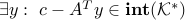 . This also implies that the primal problem is attained.
item
If both the primal and dual are strictly feasible then both are attained (and
. This also implies that the primal problem is attained.
item
If both the primal and dual are strictly feasible then both are attained (and  ).
end{itemize}
).
end{itemize}
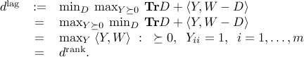
KKT conditions
Assume and both the primal and dual are attained by some primal-dual triplet  . Then,
The last term in the fourth line is equal to zero which implies  .
.
Thus the KKT conditions are:
- ,
 ,
,  ,
, ,
, , that is,
 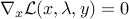 .
.
Eliminating from the above allows us to get rid of the Lagrangian stationarity condition, and gives us the following theorem.
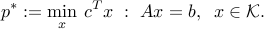
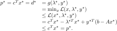
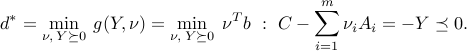
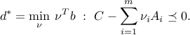
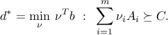
The conic problem
admits the dual bound  , where

If both problems are strictly feasible, then the duality gap is zero:  , and both values are attained. Then, a pair
  is primal-dual optimal if and only if the KKT conditions
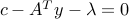
Primal feasibility:
, ,Dual feasibility:
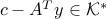 ,
,Complementary slackness:
 ,
hold.
,
hold.
SDP duality
In this section, we consider the SDP in standard form:

where  are given symmetric matrices,
  denotes the scalar product between two symmetric matrices, and
  is given.
Conic Lagrangian
Consider the ‘‘conic’’ Lagrangian
where now we associate a matrix dual variable  to the constraint
  .
.
Let us check that the Lagrangian above ‘‘works’’, in the sense that we can represent the constrained maximization problem (ref{eq:SDP-conic:L13}) as an unconstrained, maximin problem:
We need to check that, for an arbitrary matrix  , we have

This is an immediate consequence of the following:

where we have exploited the representation of the minimum eigenvalue. The geometric interpretation is that the cone of positive-semidefinite matrices has a  angle at the origin.
Dual problem
The minimax inequality then implies
The corresponding dual function is

The dual problem then writes
After elimination of the variable , we find the dual
which is in standard inequality form.
Weak and strong duality
For the maximization problem (ref{eq:SDP-conic:L13}), weak duality states that  . Note that the fact that weak duality inequality
holds for any primal-dual feasible pair  , is a direct consequence of (ref{eq:conic-dual-SDP-L13}).
From Slater’s theorem, strong duality will hold if the primal problem is strictly feasible, that is, if there exist  such that
  ,
,  .
It turns out that if both problems are strictly feasible, then both problems are attained (optimal set is not empty).
.
It turns out that if both problems are strictly feasible, then both problems are attained (optimal set is not empty).
The following strong duality theorem summarizes our results.
Consider the SDP

and its dual
The following holds:
Duality is symmetric, in the sense that the dual of the dual is the primal.
Weak duality always holds:
, so that, for any primal-dual feasible pair , we have  .
.If the primal (resp.dual) problem is bounded above (resp. below), and strictly feasible, then
 and the dual (resp. primal) is attained.
If both problems are strictly feasible, then
and both problems are attained.
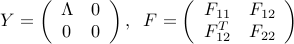
KKT conditions
Consider the SDP

with  ,
,  ,
,  . The Lagrangian is
(
. The Lagrangian is
(
{cal L}(x,Y) = c^Tx - mbox{bf Tr} F(x) Y,
)
and the dual problem reads

The KKT conditions for optimality are as follows:
 ,
, ,
,  ,
,  ,
, .
.
The last condition can be expressed as  , according to the following result: Let
  . If
. If  and
and  then
then  is equivalent to
  .
.
Proof: Let  be the square root of (the unique positive semi-definite solution to
  ). We have
  , where
 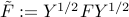 . Since , we have
  . The trace of
  being zero then implies that
  .
.
Using the eigenvalue decomposition, we can reduce the problem to the case when is diagonal. Let us assume that
where  is diagonal, and contains the eigenvalues of , and the matrix
  is of the same size as
  (which is equal to the rank of ). The condition
 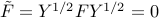 expresses as

Since  , we obtain
  . But then implies
  (use Schur complements), thus
as claimed. Thus the last KKT condition can be written as  .
.
The SDP
admits the dual bound , where

If both problems are strictly feasible, then the duality gap is zero: , and both values are attained. Then, a pair  is primal-dual optimal if and only if the KKT conditions
Primal feasibility:
,Dual feasibility:
 ,
,Complementary slackness:
 ,
hold.
,
hold.
Recall LP duality for a problem of the from  with dual variables
  has the KKT conditions were
  . This can be compactly written as
  which is similar to the KKT conditions for SDP (with
  ). This should come as no surprise as SDP problems include LP problems as a special case.
SOCP duality
We start from the second-order cone problem in inequality form:

where ,  ,
,  ,
,  ,
,  ,
,  .
.
Conic Lagrangian
To build a Lagrangian for this problem, we use the fact that, for any pair  :
:

The above means that the second-order cone has a angle at the origin. To see this, observe that
The objective in the right-hand side is proportional to the cosine of the angle between the vectors involved. The largest angle achievable between any two vectors in the second-order cone is . If  , then the cosine reaches negative values, and the maximum scalar product becomes infinite.
|
|
Geometric interpretation of the |
Consider the following Lagrangian, with variables  ,
,  ,
,  , :
, :
![{cal L}(x,lambda,u_1,ldots,u_m) = c^Tx - sum_{i=1}^m left[ u_i^T(A_ix+b_i) + lambda_i (c_i^Tx+d_i) right].](eqs/1790459814856043096-130.png)
Using the fact above leads to the following minimax representation of the primal problem:

Conic dual
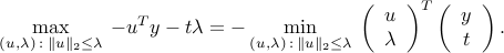
Weak duality expresses as , where

The inner problem, which corresponds to the dual function, is very easy to solve as the problem is unconstrained and the objective affine (in ). Setting the derivative with respect to leads to the dual constraints
![c=sum_{i=1}^m [A_i^Tu_i + lambda_i c_i ].](eqs/240131034187988356-130.png)
We obtain
![d^ast = max_{lambda,u_i, : i=1,ldots,m} : -lambda^Td - sum_{i=1}^m u_i^Tb_i ~:~ c=sum_{i=1}^m [A_i^Tu_i + lambda_i c_i ] , ;; |u_i|_2 le lambda_i, ;; i=1,ldots,m.](eqs/6018559603529442561-130.png)
The above is an SOCP, just like the original one.
Direct approach
As for the SDP case, it turns out that the above “conic” approach is the same as if we had used the Lagrangian
![{cal L}_{rm direct}(x,lambda) = c^Tx + sum_{i=1}^m lambda_i left[ |A_ix+b_i|_2- (c_i^Tx+d_i) right].](eqs/6049346043890555166-130.png)
Indeed, we observe that

Strong duality for SOCPs
Strong duality results are similar to those for SDP: a sufficient condition for strong duality to hold is that one of the primal or dual problems is strictly feasible. If both are, then the optimal value of both problems is attained.
Consider the SOCP

and its dual
The following holds:
Duality is symmetric, in the sense that the dual of the dual is the primal.
Weak duality always holds:
, so that, for any primal-dual feasible pair  , we have
  .
.If the primal (resp. dual) problem is bounded above (resp. below), and strictly feasible, then
and the dual (resp. primal) is attained.If both problems are strictly feasible, then
and both problems are attained.
Examples
Largest eigenvalue problem
Let us use the KKT conditions to prove that, for any given matrix  :
:

where  denotes the largest singular value.
Duality theory for SDP immediately tells us that the second equality holds. Indeed, the SDP

admits the following dual (see XXX):
Using the eigenvalue decomposition of  , it is easy to show that
  .
.
It remains to prove the first equality. We observe that

(To see this, set  .) Thus we need to show that at optimum, the rank of the primal variable
  in the problem above is one.
The pair of primal and dual problems are both strictly feasible, hence the KKT condition theorem applies, and both problems are attained by some primal-dual pair  , which satisfies the KKT conditions. These are ,
  , and
, and  . The last condition proves that any non-zero column of satisfies
  (in other words, is an eigenvector associated with the largest eigenvalue). Let us normalize so that
  , so that
  . We have
  , which proves that the feasible primal variable
  ,
,  , is feasible and optimal for the primal problem (ref{eq:primal-evpb-L15}). Since
  has rank one, our first equality is proved.
An SDP where strong duality fails
Contrarily to linear optimization problems, SDPs can fail to have a zero duality gap, even when they are feasible. Consider the example:
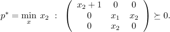
Any primal feasible satisfies  . Indeed, positive-semidefiniteness of the lower-right
  block in the LMI of the above problem writes, using Schur complements, as
  ,
,  . Hence, we have
  . The dual is

Any dual feasible satisfies  (since
  ), thus
 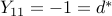 .
.
An eigenvalue problem
For a matrix  , we consider the SDP

The associated Lagrangian, using the conic approach, is

with the matrix dual variable , while  is free.
The dual function is
We obtain the dual problem

Eliminating leads to

Both the primal and dual problems are strictly feasible, so , and both values are attained. This proves the representation given above for the largest eigenvalue of .
SDP relaxations for a non-convex quadratic problem
In XXx, we have seen two kinds of relaxation for the non-convex problem

where the symmetric matrix  is given.
One relaxation is based on a standard relaxation of the constraints, and leads to (see XXX)

Another relaxation (XXX) involved expressing the problem as an SDP with rank constraints on the a matrix :

Let us examine the dual of the first relaxation (ref{eq:lag-rel-sdp-bool-L13}). We note that the problem is strictly feasible, so strong duality holds. Using the conic approach, we have
This shows that both Lagrange and rank relaxations give the same value, and are dual of each other.
In general, for arbitrary non-convex quadratic problems, the rank relaxation can be shown to be always better than the Lagrange relaxation, as the former is the (conic) dual to the latter. If either is strictly feasible, then they have the same optimal value.
Minimum distance to an affine subspace
Return to the problem seen in XXX:

where  ,
,  , with
  in the range of . We have seen how to develop a dual when the objective is squared. Here we will work directly with the Euclidean norm.
The above problem is an SOCP. To see this, simply put the problem in epigraph form. Hence the above theory applies. A more direct (equivalent) way, which covers cases when norms appear in the objective, is to use the representation of the objective as a maximum:

The dual function is
We obtain the dual
Eliminating  :
:
Robust least-squares
Consider a least-squares problem
where  , . In practice, may be noisy. To handle this, we assume that is additively perturbed by a matrix bounded in largest singular value norm (denoted
  in the sequel) by a given number
  . The robust counterpart to the least-squares problem then reads
Using convexity of the norm, we have

The upper bound is attained, with the choicefootnote{We assume that  ,
,  . These cases are easily analyzed and do not modify the result.}
Hence, the robust counterpart is equivalent to the SOCP
Again, we can use epigraph representations for each norm in the objective:

and apply the standard theory for SOCP developed in section ref{s:dual-pb-socp-L14}. Strong duality holds, since the problem is strictly feasible.
An equivalent, more direct approach is to represent each norm as a maximum:

Exchanging the min and the max leads to the dual

The dual function is

Eliminating , we obtain the dual

As expected, when  grows, the dual solution tends to the least-norm solution to the system . It turns out that the above approach leads to a dual that is equivalent to the SOCP dual, and that strong duality holds.
Probabilistic classification
Consider a binary classification problem, in which the data points for each class and radom variables  , each assumed to obey to a given Gaussian distribution
  , where
  ,
,  are the given class-dependent means and covariance matrices, respectively. We seek an hyperplane
  that probabilistically separates the two classes, in the sense that

where  is a given small number. The interpretation is that we would like that, with high probability, the samples taken from each distribution fall on the correct side of the hyperplane. The number
  allows to set the level of reliability of the classification, with small corresponding to a low probability of mis-classification. We assume that
  .
.
When obeys to a distribution  , the random variable
  follows the distribution
  , with
  ,
,  . We can write
  , with a normal (zero-mean, unit variance) random variable. We thus have

where  is the cumulative density function of the normal distribution, namely
  . Since is monotone increasing, the condition
  is equivalent to
  , or
, or  , where
  . Note that
  whenever
  .
.
We obtain that the probability constraints above write

Note that when  , he above simply requires the correct classification of the means
  . When
  grows in size, he conditions become more and more stringent. We can eliminate from the constraints above: these constraints hold for some if and only if

Let us minimize the error probability level . Since  is decreasing in , we would like to maximize subject to the constraints above. Exploiting homogeneity, we can always require
  . We are led to the problem

This is an SOCP, which is strictly feasible (in the sense of weak Slater’s condition), since . Hence strong duality holds.
The dual can be obtained from the minimax expression

Exchanging the min and max yields

We observe that  at the optimum, otherwise we would have , which is clearly impossible when . We then set
  , scale the variables
  by
by  , and change
  into its opposite. This leads to the dual

The geometric interpretation is as follows. Consider the ellipsoids  . The constraints in the dual problem above state that these two ellipsoids intersect. The dual problem amounts to finding the smallest for which the two ellipsoids
  intersect. The optimal value of
  is then
  , and the corresponding optimal value of the error probability level is
  . It can be shown that the optimal separating hyperplane corresponds to the common tangent at the intersection point.