Weak Duality

Lagrange dual problem
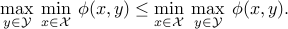
Weak duality and minimax inequality
Examples

Lagrange dual problem

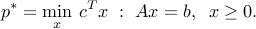
Primal problem

In this section, we consider a possibly non-convex optimization problem
$p^ast := displaystylemin_x : f_0(x) ~:~ begin{array}[t]{l} f_i(x) le 0,quad i=1,cdots, m, % h_i(x) = 0, quad i=1,cdots,p, end{array}$
where the functions f_0,f_1,ldots,f_m

We denote by {cal D}

the domain of the problem (which is the intersection of the domains of all the functions involved), and by {cal X} subseteq {cal D}

its feasible set.

We will refer to the above as the primal problem, and to the decision variable

in that problem, as the primal variable. One purpose of Lagrange duality is to find a lower bound on a minimization problem (or an upper bounds for a maximization problem). Later, we will use duality tools to derive optimality conditions for convex problems.

Lagrangian

To the problem we associate the Lagrangian ${cal L} : mathbf{R}^n times mathbf{R}^m rightarrow mathbf{R}$ , with values
${cal L}(x,lambda) : = f_0(x) + sum_{i=1}^m lambda_i f_i(x) ,$
where the new variables $lambda in mathbf{R}^m$ , are called Lagrange multipliers, or dual variables.

We observe that, for every feasible x in {cal X}

, and every lambda ge 0

is bounded below by {cal L}(x,lambda)

:
$forall : x in {cal X}, ;; forall : lambda in mathbf{R}_+^m ~:~ f_0(x) ge {cal L}(x,lambda).$

The Lagrangian can be used to express the primal problem (ref{eq:convex-pb-L11}) as an unconstrained one. Precisely:
$p^ast = min_x : max_{lambda ge 0} : {cal L}(x,lambda),$
where we have used the fact that, for any vector $f in mathbf{R}^m$ , % $h in mathbf{R}^p$ , we have
$max_{lambda ge 0} : lambda^Tf = left{ begin{array}{ll} 0 & mbox{if } f le 0 +infty & mbox{otherwise.} end{array} right.$

Lagrange dual function

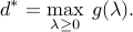
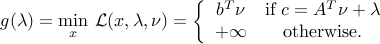
We then define the Lagrange dual function (dual function for short) as the function with values
$g(lambda) := min_x : {cal L}(x,lambda) .$
Note that, since

is the point-wise minimum of affine functions ( {cal L}(x,cdot)

is affine for every

), it is concave. Note also that it may take the value -infty

From the bound above, by minimizing over

in the right-hand side, we obtain
$forall : x in {cal X}, ;; forall : lambda ge 0 ~:~ f_0(x) ge min_{x'} : {cal L}(x',lambda,) = g(lambda),$
which, after minimizing over

the left-hand side, leads to the lower bound
$forall : lambda in mathbf{R}_+^m ~:~ p^ast ge g(lambda).$

Lagrange dual problem

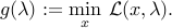
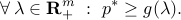
The best lower bound that we can obtain using the above bound is p^ast ge d^ast

, where
$d^ast = max_{lambda ge 0} : g(lambda).$
We refer to the above problem as the dual problem, and to the vector $lambda in mathbf{R}^m$ as the dual variable. The dual problem involves the maximization of a concave function under convex (sign) constraints, so it is a convex problem. The dual problem always contains the implicit constraint lambda in mbox{bf dom} g

Case with equality constraints

If equality constraints are present in the problem, we can represent them as two inequalities. It turns out that this leads to the same dual, as if we would directly use a single dual variable for each equality constraint, which is not restricted in sign. To see this, consider the problem
$p^ast := displaystylemin_x : f_0(x) ~:~ begin{array}[t]{l} f_i(x) le 0,quad i=1,cdots, m, h_i(x) = 0, quad i=1,cdots,p. end{array}$
We write the problem as
$p^ast := displaystylemin_x : f_0(x) ~:~ begin{array}[t]{l} f_i(x) le 0,quad i=1,cdots, m, h_i(x) le 0, ;; -h_i(x) le 0, quad i=1,cdots,p. end{array}$
Using a multiplier nu_i^pm

for the constraint pm h_i(x) le 0

, we write the associated Lagrangian as
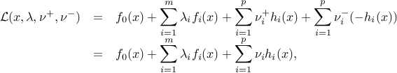
$begin{array}{rcl}{cal L}(x,lambda,nu^+,nu^-) &=& f_0(x) + displaystylesum_{i=1}^m lambda_i f_i(x) + sum_{i=1}^p nu_i^+ h_i(x) + displaystylesum_{i=1}^p nu_i^-(- h_i(x)) &=& f_0(x) + displaystylesum_{i=1}^m lambda_i f_i(x) + sum_{i=1}^p nu_i h_i(x) , end{array}$
where nu := nu^+-nu^-

does not have any sign constraints.

Thus, inequality constraints in the original problem are associated with sign constraints on the corresponding multipliers, while the multipliers for the equality constraints are not explicitly constrained.

Weak duality and minimax inequality

Weak duality theorem

Theorem: weak duality

For a general (possibly non-convex) problem
$p^ast := displaystylemin_x : f_0(x) ~:~ begin{array}[t]{l} f_i(x) le 0,quad i=1,cdots, m, h_i(x) = 0, quad i=1,cdots,p , end{array}$
weak duality holds: p^ast ge d^ast .

Geometric interpretation

Assume that there is only one inequality constraint in the primal problem ( m=1

), and let (

{cal G} := left{ (f_1(x),f_0(x)) : x in mathbf{R}^n right}. ) We have
$p^ast = min_{u,t} : t ~:~ (u,t) in {cal G} , ;; u le 0 .$
and
$g(lambda) = min_{u,t} : (lambda,1)^T(u,t) ~:~ (u,t) in {cal G} .$
If the minimum is finite, then the inequality (lambda,1)^T(u,t) ge g(lambda)

defines a supporting hyperplane, with slope -lambda

, of

. (See Figs. 5.3 and 5.4 in BV,p.233.)

Minimax inequality

Weak duality can also be obtained as a consequence of the following minimax inequality, which is valid for any function phi

of two vector variables x,y

, and any subsets {cal X}

:
$max_{y in {cal Y}} : min_{x in {cal X}} : phi(x,y) le min_{x in {cal X}} : max_{y in {cal Y}} : phi(x,y).$
To prove this, start from
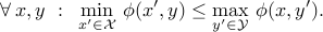
$forall : x, y ~:~ min_{x' in {cal X}} : phi(x',y) %le {cal L}(x,y) le max_{y' in {cal Y}} : phi(x,y').$
and take the minimum over xin {cal X}

on the right-hand side, then the maximum over yin {cal Y}

on the left-hand side.

Weak duality is indeed a direct consequence of the above. To see this, start from the unconstrained formulation (ref{eq:pb-primal-unconstr-L11}), and apply the above inequality with phi = {cal L}

the Lagrangian of the original problem, and y=lambda

the vector of Lagrange multipliers.

Interpretation as a game

We can interpret the minimax inequality result in the context of a one-shot, zero-sum game. Assume that you have two players A and B, where A controls the decision variable

, while B controls

. We assume that both players have full knowledge of the other player’s decision, once it is made. The player A seeks to minimize a payoff (to player B) {cal L}(x,y)

, while B seeks to maximize that payoff. The right-hand side in (ref{eq:min-max-theorem-L11}) is the optimal pay-off if the first player is required to play first. Obviously, the first player can do better by playing second, since then he or she knows the opponent’s choice and can adapt to it.

Examples

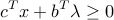
Linear optimization problem, inequality form

Consider the LP in standard inequality form
p^ast = min_x : c^Tx ~:~ Ax le b,

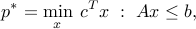
where $A in mathbf{R}^{m times n}$ , $b in mathbf{R}^m$ , and the inequality in the constraint Ax le b

is interpreted component-wise.

{cal L}(x,lambda) = c^Tx + lambda^T(Ax-b) ) and the corresponding dual function is
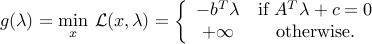
$g(lambda) = min_x : {cal L}(x,lambda) = left{ begin{array}{cc} -b^Tlambda & mbox{if } A^Tlambda + c = 0 +infty & mbox{otherwise.} end{array}right.$
The dual problem reads
d^ast = max_lambda : g(lambda) = max_lambda : -b^Tlambda ~:~ lambda ge 0, ;; A^Tlambda + c = 0.

d^ast = max_lambda : g(lambda) = max_lambda : -b^Tlambda ~:~ lambda ge 0, ;; A^Tlambda + c = 0.

The dual problem is an LP in standard (sign-constrained) form, just as the primal problem was an LP in standard (inequality) form.

Weak duality implies that
c^Tx + b^Tlambda ge 0

for every

such that

. This property can be proven directly, by replacing

in the left-hand side of the above inequality, and exploiting Ax le b

and

Linear optimization problem, standard form

We can also consider an LP in standard form:
p^ast = min_x : c^Tx ~:~ Ax = b, ;; x ge 0.

The equality constraints are associated with a dual variable

that is not constrained in the dual problem.

The Lagrange function is
${cal L}(x,lambda,nu) = c^Tx - lambda^Tx + nu^T(b-Ax)$
and the corresponding dual function is
$g(lambda) = min_x : {cal L}(x,lambda,nu) = left{ begin{array}{cc} b^Tnu & mbox{if } c = A^Tnu +lambda +infty & mbox{otherwise.} end{array}right.$
The dual problem reads
$d^ast = max_{lambdage 0,: nu}: g(lambda,nu) = max_nu : b^Tnu ~:~ c ge A^Tnu .$
This is an LP in inequality form.

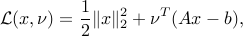
Minimum Euclidean distance problem

Consider the problem of minimizing the Euclidean distance to a given affine space:
$min: frac{1}{2} |x|_2^2 ~:~ Ax = b,$
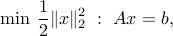
where $A in mathbf{R}^{p times n}$ , $b in mathbf{R}^p$ . We assume that

is full row rank, or equivalently, AA^T succ 0

. The Lagrangian is
${cal L}(x,nu) = frac{1}{2} |x|_2^2 + nu^T(Ax-b),$
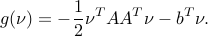
and the Lagrange dual function is
$g(nu) = min_x : {cal L}(x,nu) = min_x : frac{1}{2} |x|_2^2 + nu^T(Ax-b).$
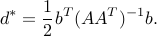
In this example, the dual function can be computed analytically, using the optimality condition $nabla_x {cal L}(x,nu) = x + A^Tnu = 0$ . We obtain x = -A^Tnu

, and
$g(nu) = -frac{1}{2} nu^TAA^Tnu - b^T nu.$
The dual problem expresses as
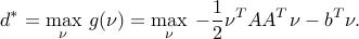
$d^ast = max_nu : g(nu) = max_nu : -frac{1}{2} nu^TAA^Tnu - b^T nu.$
The dual problem can also be solved analytically, since it is unconstrained (the domain of

is the entire space $mathbf{R}^p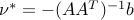$ ). We obtain $nu^ast = -(AA^T)^{-1} b$ , and
$d^ast = frac{1}{2} b^T(AA^T)^{-1} b.$
We have thus obtained the bound p^ast ge d^ast

A non-convex boolean problem

For a given matrix W=W^T succ 0

, we consider the problem
p^ast = max_x : x^TWx ~:~ x_i^2 le 1, i=1,ldots,n.

In this maximization problem, Lagrange duality will provide an upper bound on the problem. This is called a ‘‘relaxation’’, as we go above the true maximum, as if we’d relax (ignore) constraints.

The Lagrangian writes
${cal L}(x,lambda) = x^TWx + sum_{i=1}^n lambda_i (1-x_i^2) = mbox{bf Tr} D_lambda + x^T(W-D_lambda)x.$
where $D_lambda := mbox{bf diag}(lambda)$ .

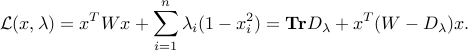
To find the dual function, we need to maximize the Lagrangian with respect to the primal variable

. We express this problem as
$g(lambda) = max_x : {cal L}(x,lambda) = min_t : t ~:~ forall : x , ;; t ge mbox{bf Tr} D_lambda + x^T(W-D_lambda)x .$
The last inequality holds if and only if
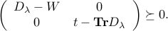
$left( begin{array}{cc} D_lambda-W & 0 0 & t-mbox{bf Tr} D_lambda end{array}right) succeq 0.$
Hence the dual function is the optimal value of an SDP in one variable:
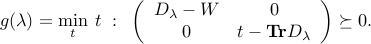
$g(lambda) = min_t : t ~:~ left( begin{array}{cc} D_lambda-W & 0 0 & t-mbox{bf Tr} D_lambda end{array}right) succeq 0.$
We can solve this problem explicitly:
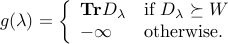
$g(lambda) = left{ begin{array}{ll}mbox{bf Tr} D_lambda &mbox{if } D_lambda succeq W -infty & mbox{otherwise.} end{array}right.$
The dual problem involves minimizing (that is, getting the best upper bound) the dual function over the variable lambda ge 0

:
$d^ast = min_{lambda} : lambda^Tmathbf{1}~:~ mbox{bf diag}(lambda) succeq W .$
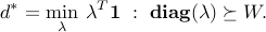
The above is an SDP, in variable lambda

. Note that lambda > 0

is automatically enforced by the PSD constraint.

The Lagrange relaxation of the primal problem can be interpreted geometrically, as follows.