Computational Photography: Autostitching and Photomosaics - Part B
Aneesh Akella
Introduction
This project is about automating mosaic production. To see, manual mosaic production please click here.
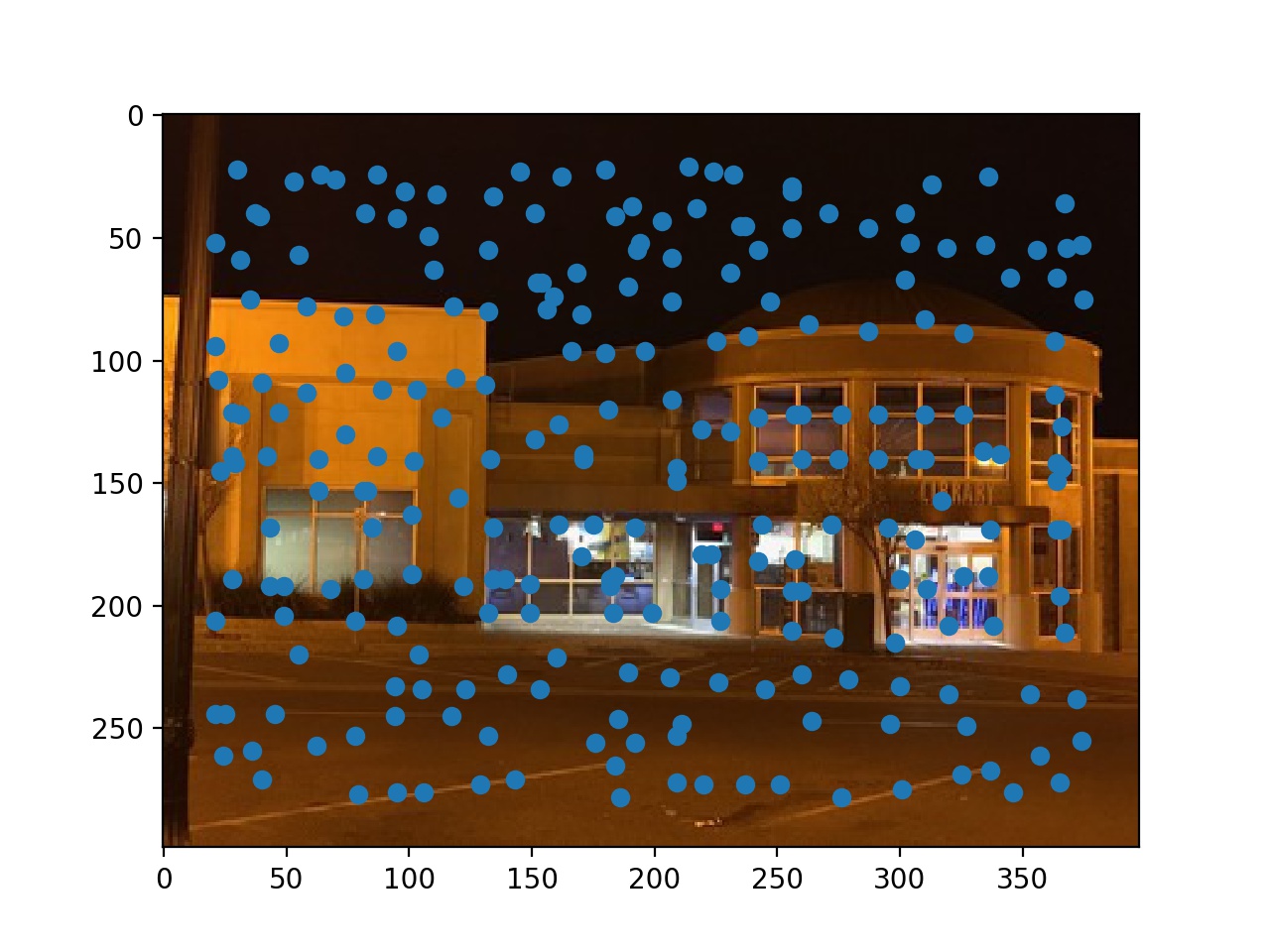
Harris Corners and Adaptive Non Maximal Suppression (ANMS)
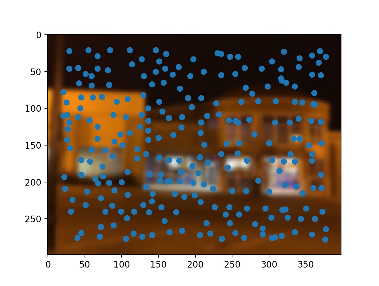
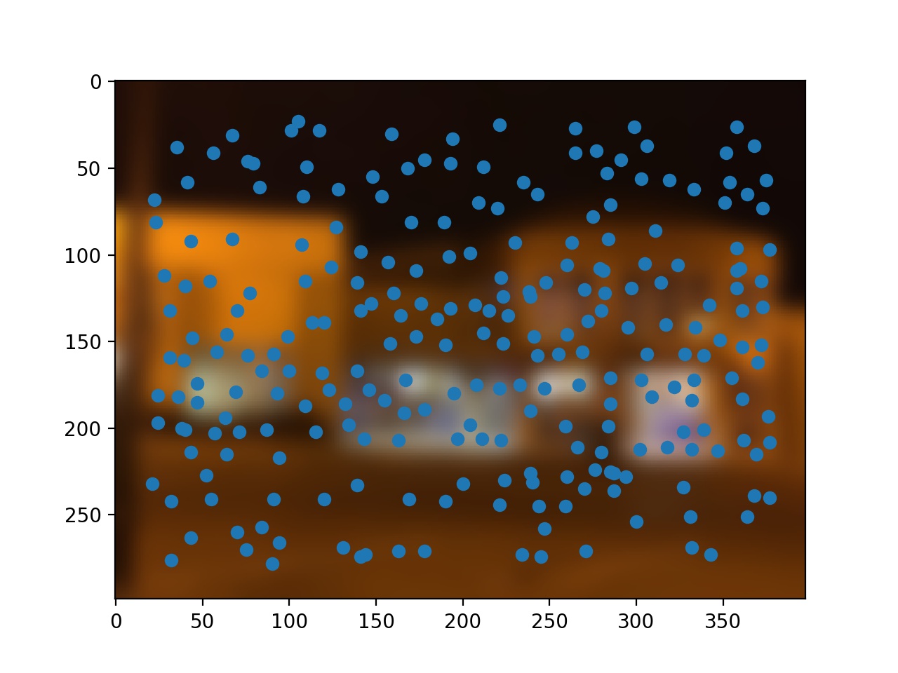
Using strictly the Harris Corner algorithm, one can see that there are too many points. Thus, we need a way of reducing the number of points.
This is why we need adaptive non-maximal supression.
For a given point, the algorithm determines the closest point that has a Harris Score that is at least 1⁄c
times greater than the Harris Score for the given point. Once each point's Harris partner has been found, the radius between the two is calculated. We choose between 100-500 points of points with the highest non-maximal supression radius to ensure an even spread.The greater the c, the larger the supression radius, and the wider the spread. We want multiple points with decent spread so we chose 0.9 as c.
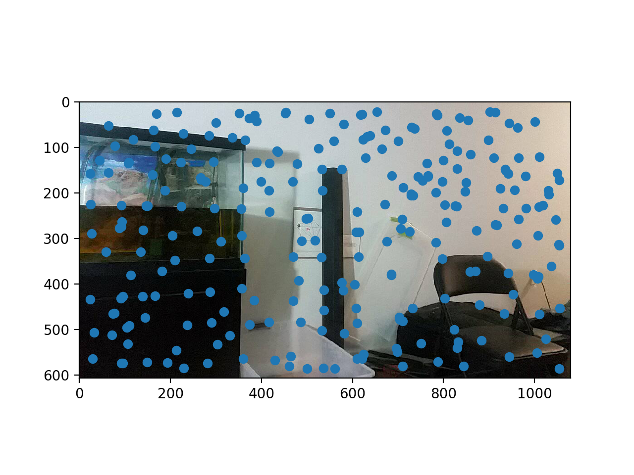
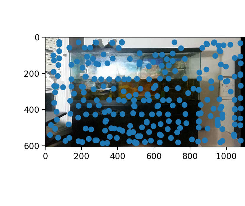
Before ANMS
Left Image: Around 15000 points
Right Image: Around 15000 points
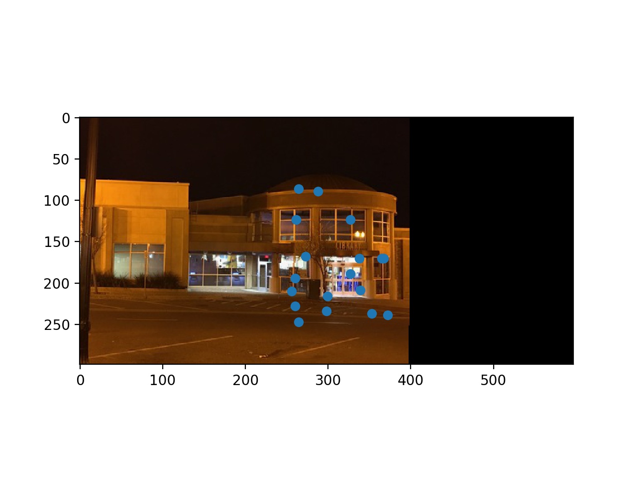
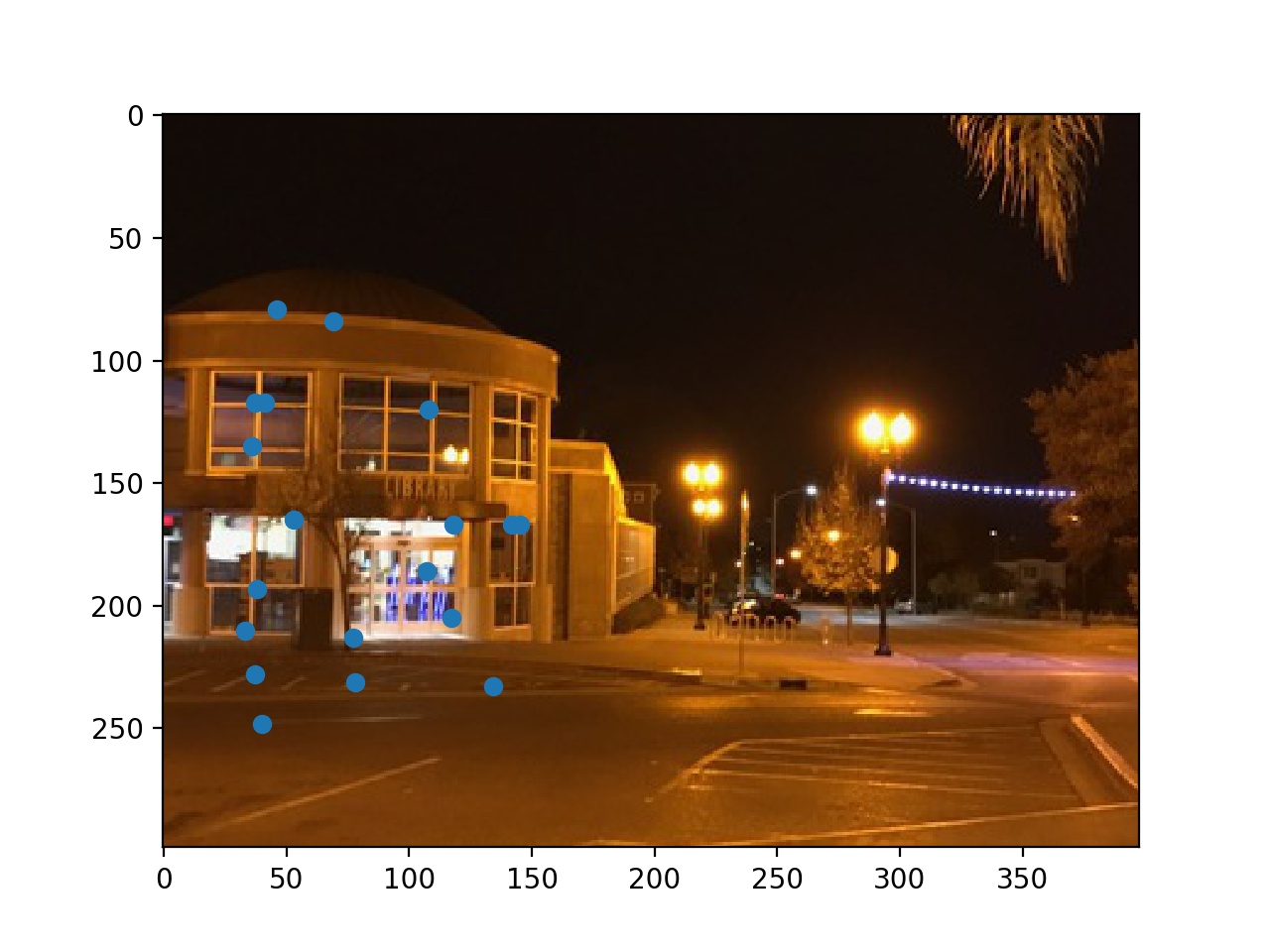
After ANMS
Left Image: 250 points
Right Image: 250 points
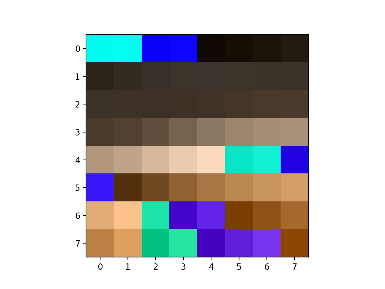
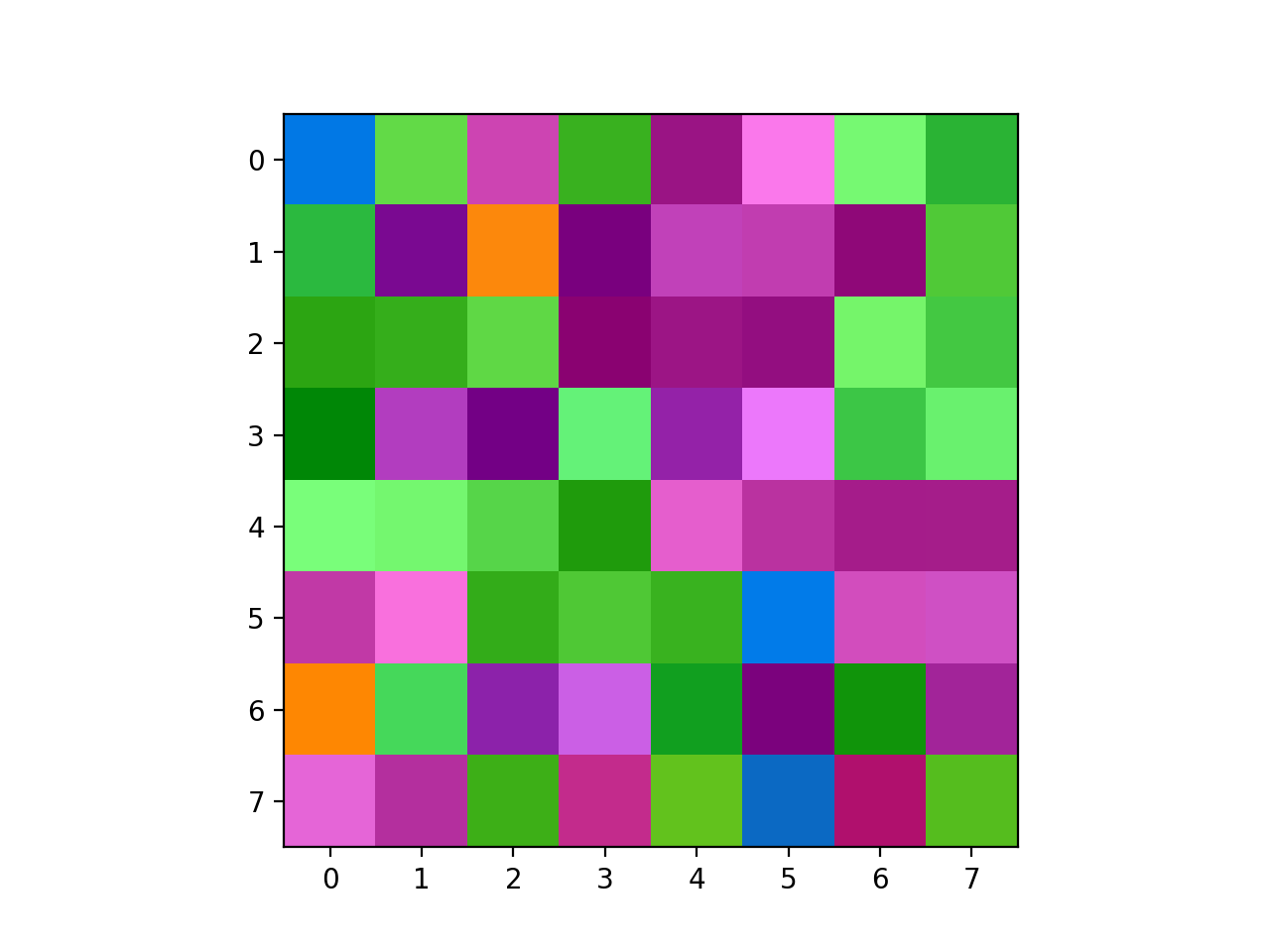
Feature Descriptor
Now that the points are evenly spread a question lies: How do we match points on different images to each other? Simply put, we take a 40 * 40 patch around each point, reduce the size to an 8 * 8 patch, and bias/gain normalize the picture. Normalizing and reducing the size lessens the impact of higher frequencies and varying intensities. Then, we match each feature to feature within the two images. If two features within different images have an SSD of less than 0.3, we consider it a match. However, there is the possibility of outliers, which we will get to next.
Feature Descriptor Examples
RANSAC
In the RANSAC algorithm, we choose 4 random corresponding points from each point and compute the homography. Then for a point on each image, we multiply the homography matrix and see if it is within 10 pixels of its corresponding point. If this is true, it is considered an inlier and added to a list of inliers. This algorithm is run 10000 times and the result is a massive list of lists of inliers. We search for the list that has the most entries in it along with the homography matrix that produced this list. The homography that produces the most inliers will be used to reconstruct the projective transformation.
Potential Inliers
Left Side Inliers
Right Side Inliers
Mosiacs
Ulitmately, the algorithm aligned the pictures very well. It aligned some even better than I could manually like the fountain mosaic.
Here are the mosaics:
Fish Tank
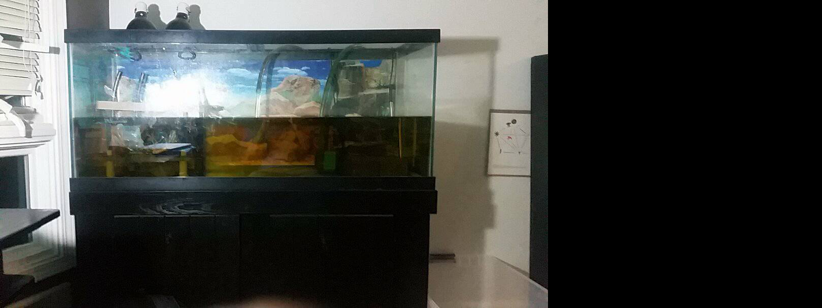
Left Warped
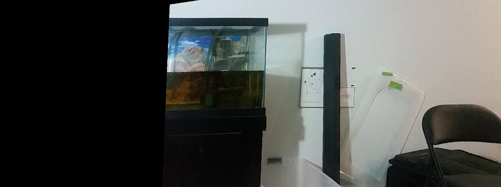
Right Warped
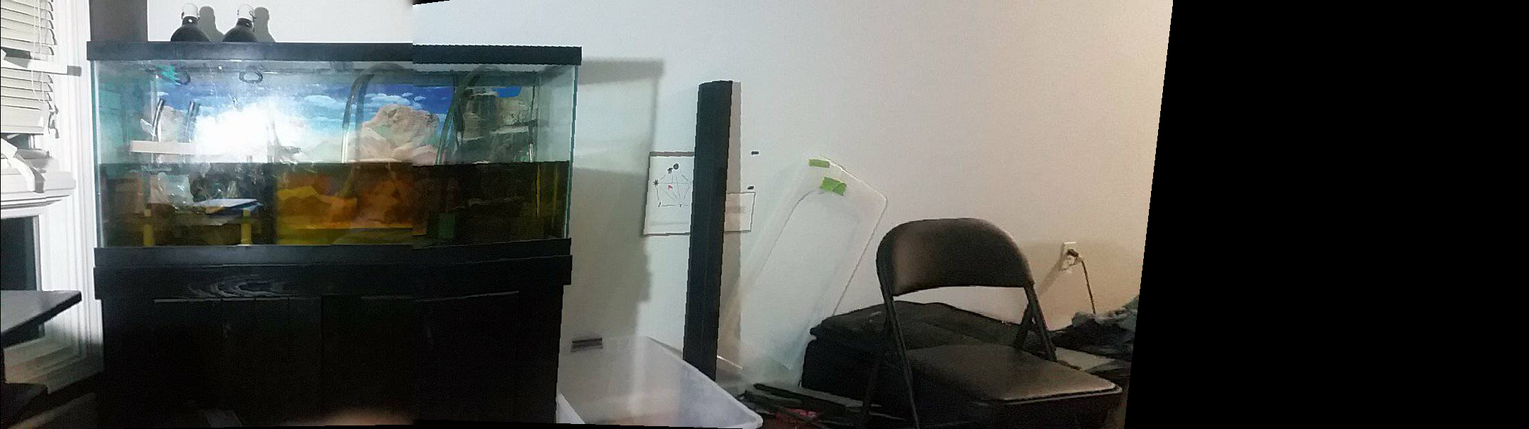
Manual
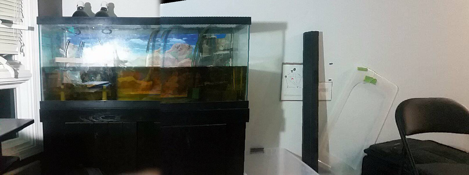
Autowarped
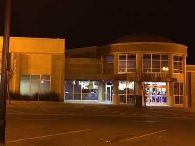
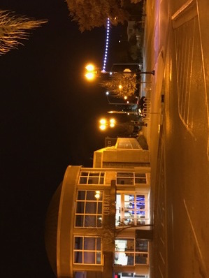
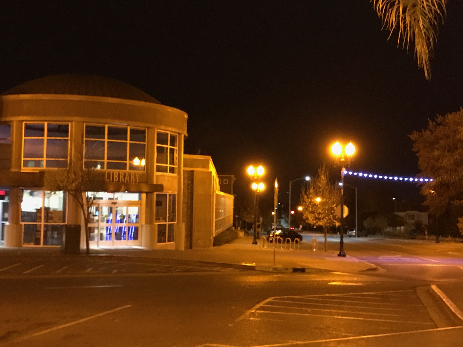
Library
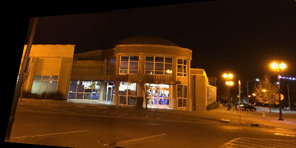
Manual
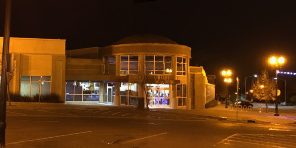
Autowarped
Fountain
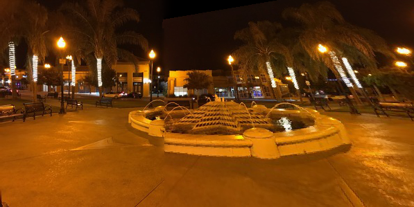
Manual
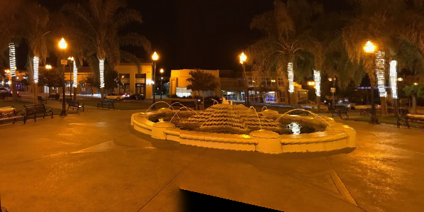
Autowarped
Bells and Whistles: Auto Panorama Recognition
Provided an input image, my algorithm looks through each image in its dictionary. If there is a picture with more than 6 inliers, this corresponding image is returned as a match. Weighted average blending is then used to stich the pictures togther. Additional features we added to prevent the edge case where left and right images were mixed up. To implement this, I always warped the right image to the left image. The input image is a right image, however, the algorithm either way created the right result.
Input Photo

List of Images
]

Blended Result
Bells and Whistles: Gif Homography
A combination of Project 6 and Project 3: Ultimately, the homography between all images does not change. Therefore, we can compute an array of photos and transform this into a gif using the same homography.
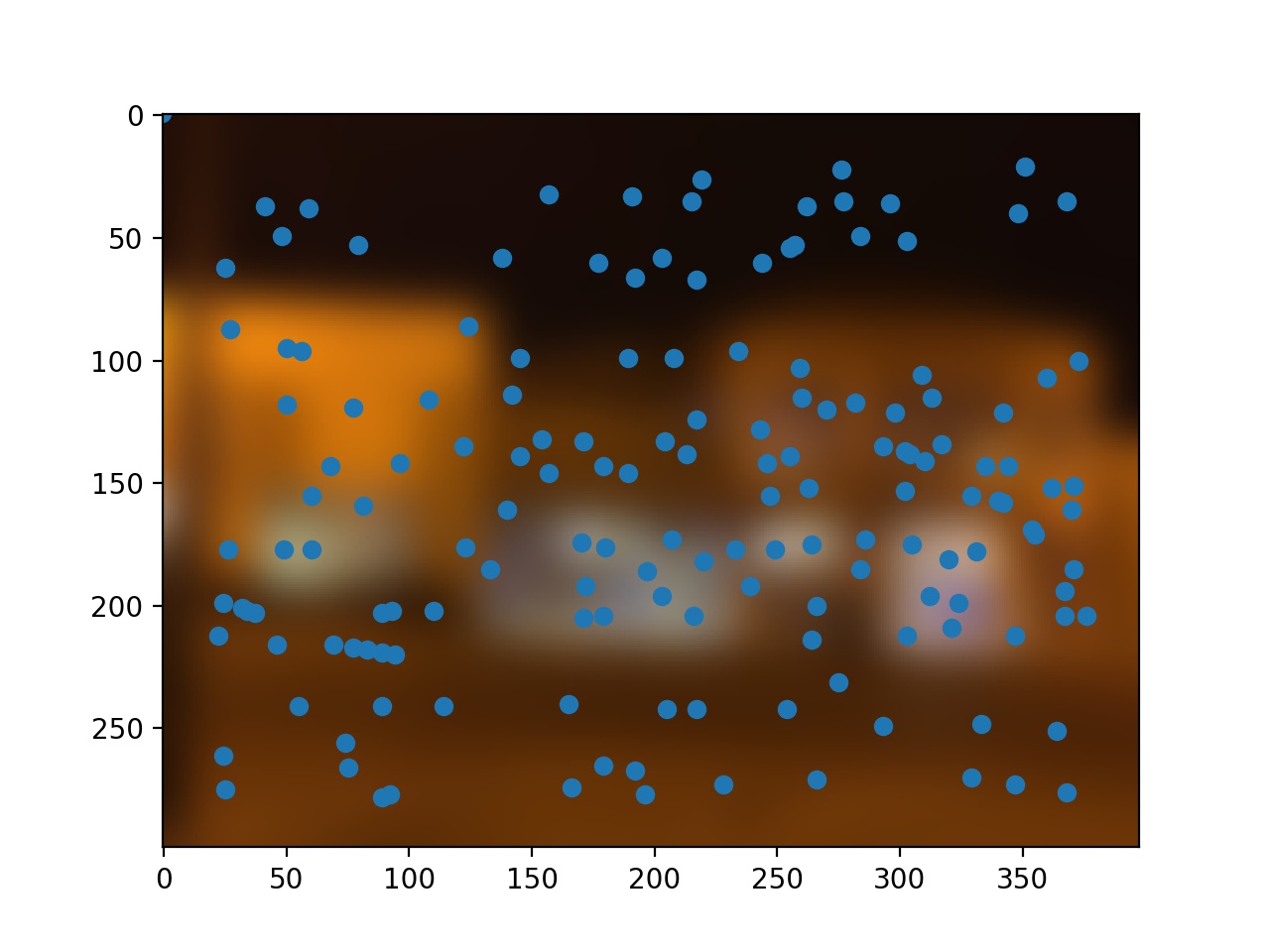
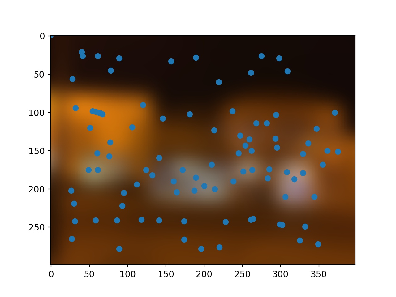
Using a Gaussian pyramid, we blur the image at several levels and run ANMS on each image. As you can see, the number of corners reduces tremendously as the images get blurrier and blurrier. This can be utilized to detect more accurate features and corners between images.
To make a feature rotationaly invariant, the x-and y gradients are calculated and the angle arctan((d/dy)/(d/dx)) is calculated as well. After this orientation is calculated, we normalize the orientation by rotating the patch so the orientation is the same.