Project 2: Fun with Filters and Frequencies!
1 Fun with Filters
1.1 Finite Difference Operator
In this section the camera man image in Figure 1 was convolved with finite difference operators defined as:
\(D_x = \begin{bmatrix} 1 -1\end{bmatrix}\) , \(D_y = \begin{bmatrix}1 \\-1\end{bmatrix}\)
to get partial derivatives of the camera man image (Efros and Kanazawa, 2021).

Figure 1: Camera Man


Figure 2: a)Partial Derivative wrt x b)Partial Derivative wrt y


Figure 3: a)Gradient Maganitude Image b) Binarized Gradient Maganitude Image
Figure 2.a. and 2.b. represent the partial derivative with respect to (wrt) \(x\) and \(y\), respectively. The Partial derivative wrt \(x\) is given by \(\frac{\partial f(x,y)}{\partial x}\), and by definition it captures the change in the image intensity as \(x\) changes. This is why the vertical lines of the image are more prominent in Figure 2.a. Whereas the partial derivative wrt \(y\), given by \(\frac{\partial f(x,y)}{\partial y}\), captures horizontal line on an image, as observed in Figure 2.b.
Combining the partial derivatives of an image into a vector gives you the image gradient, which is defined as :
\[ \nabla f = \begin{bmatrix}\frac{\partial f(x,y)}{\partial x}, \frac{\partial f(x,y)}{\partial y} \end{bmatrix}\] (Szeliski, 2020)
The gradient of an image points in the direction that experiences rapid change in intensity. Computing \(L_2-norm\) of the image gradient captures the gradient magnitude image, shown in Figure 3.a., also known as the edge strength and is given by:
\[|| \nabla f || =\sqrt{\frac{\partial f(x,y)}{\partial x} ^2+ \frac{\partial f(x,y)}{\partial y}^2 } \] (Szeliski, 2020)
So gradient magnitude image tells us how fast the image intensity is changing and the image gradient gives us the direction in which the image is rapidly changing. The gradient magnitude image acts like an edge detector because pixels with high change( i.e. High \(\frac{\partial f(x,y)}{\partial x}\) and \(\frac{\partial f(x,y)}{\partial y}\)) have prominent white values and pixels with little or no change are black.
Figure 3.b. represents the binarized gradient magnitude image with 0.1 as the threshold. This helped us reduce noise and expose the strong edges of the image.
1.2 Derivative of Gaussian (DoG)
In this section the camera man image in Figure 1 was convolved with a Gaussian filter,and then the steps done in the previous section were repeated to compare the outputs of two approaches.
A 2D Gaussian filter was computed by using cv2.getGaussianKernel() with \(ksize=2\) and \(sigma=10\).


Figure 4: a)Partial Derivative wrt x b)Partial Derivative wrt y


Figure 5: a)Partial Derivative wrt x b)Partial Derivative wrt y


Figure 6: a)Gradient Maganitude Image b) Binarized Gradient Maganitude Image
The partial derivatives of the smoothed image captures more vertical and horizontal line the one without. There is less noise captured in the binarized gradient magnitude image for the smoothed image compared to the one without smoothing from the previous section.
There’s a theorem called the Derivative Theorem of Convolution which can help with reducing the run-time for generating gradient magnitude images. The theorem states that
\[\frac{\partial}{\partial x}(h*f) =(\frac{\partial}{\partial x}h)*f \]
(Szeliski, 2020)
This means one can perform a single convolution instead of two by creating a derivative of Gaussian filters. Figure 7 shows that the results from a single convolution and two convolutions are the same, which confirms the theorem.
Figure 7:a) Double Convolution b) Single Convolution
2 Fun with Frequencies
2.1 Image Sharpening
In this section we focus on sharpening images. We start off with sharpening blurry images by following these steps:
Apply a Gaussian filter (\(g\)) on the image of interest (\(f)\). Gaussian is a low pass filter that outputs a low frequency image (\(I_{low}\)) which is the blurry version of the original image: \[ I_{low} = f*g \]
Subtract the low frequency image from the original image (\(f\)) to get the high frequencies of the image (\(I_{high}\)):
\[ I_{high} = f - I_{low} \]
\[ I_{high} = f - f*g \]
- Lastly to make the image sharp, add the high frequencies with a factor \(\alpha\) to the original image : \[I_{sharp} = f + \alpha I_{high}\] \[ I_{sharp} = f + \alpha(f - f*g) \]
(Efros and Kanazawa, 2021)
Image Sharpening Implementation
The following parameters were used to sharpen the Taj image below:
Gauss Filter: {\(ksize =7 , sigma =2\)}
Sharpening factor:{\(\alpha =3\)}


a)Original Image b) Blurred Image


c)High Frequency Image d) Sharp Image
Additional Sharpening Example
The following parameters were used to sharpen the fox image below:
Gauss Filter: {\(ksize =7 , sigma =3\)}
Sharpening factor:{\(\alpha =2\)}


a)Original Image b) Blurred Image


c)High Frequency Image d)Sharp Image
Unsharp Mask Filter Implementation
There’s another sharpening technique called Unsharp Mask Filter defined as:
\[ (1+\alpha)f -\alpha f*g\] (Efros and Kanazawa, 2021)
We implemented the unsharp mask filter on same images from the previous section to compare the differences. There is a small improvement when using the unsharp mask filter that is observed in terms of sharpness. See below for unsharp mask filter results.
The following parameters were used to sharpen the Taj image below:
Gauss Filter: {\(ksize =7 , sigma =2\)}
Sharpening factor:{\(\alpha =2\)}

a)Original Image b) Sharp Image
The following parameters were used to sharpen the fox image below:
Gauss Filter: {\(ksize =7 , sigma =3\)}
Sharpening factor:{\(\alpha =2\)}
a)Original Image b) Sharp Image
The following parameters were used to sharpen the Lions’s Head Mountain image below:
Gauss Filter: {\(ksize =10 , sigma =5\)}
Sharpening factor:{ \(\alpha =2\)}


a)Original Image b) Sharp Image
The following parameters were used to sharpen the rhinos image below:
Gauss Filter: {\(ksize =3 , sigma =8\)}
Sharpening factor:{ \(\alpha =2\)}


a)Original Image b) Sharp Image
Blurring and Sharping a Sharp Image
A sharp image was blurred and sharpened again using the Unsharp Mask Filter to assess the performance of the image sharpening technique. From the image below it can be observed that blurring a sharp image and then applying Unsharp Mask Filter doesn’t give you the original image because high frequencies of the image were lost when it was blurred and sharpening it didn’t return the lost high frequencies. Overall, the new image looks less natural compared to the original.
The following parameters were used to sharpen the winelands image below:
Gaussian Filter to blur Original image: {\(ksize =3 , sigma =4\)}
Unsharp Mask Filter :{\(ksize =3 , sigma =4, \alpha =3\)}


a)Original Image b) Sharp Image
2.2 Image Hybrid
In this section, we created hybrid images of the numtmeg.jpg image and the DerekPicture.jpg image and other examples of hybrid images and also created corresponding log magnitude of the Fourier transform of the inputs and outputs. For extra credit, we also experiment with using color to enhance the effect.
Input Images with Corresponding log magnitude of the Fourier transform


a)DerekPicture.jpg Image b)log magnitude of the Fourier transform


a)nutmeg.jpg Image b)log magnitude of the Fourier transform
Filtered Images with Corresponding log magnitude of the Fourier transform
The following parameters were used to low pass filter the image below:
- Gaussian Filter to low pass filter the Original image: {\(ksize =15 , sigma =20\)}


Low frequency image with corresponding log magnitude of the Fourier transform
The following parameters were used to high pass filter the image below:
- Gaussian Filter to high pass filter the Original image: {\(ksize =60 , sigma =30\)}


High freqeuncy image with corresponding log magnitude of the Fourier transform
Color Enhancing Experiment
All the combinations of high and low frequency images of color and grayscale hybrid images were created. The final outcomes look different and I prefer the Hybrid Image with Low Frequency Color Image and High Frequency Grayscale Image. See Below for experiment output.
1. Hybrid Image of Low Frequency Color Image and High Frequency Grayscale Image


Hybrid image of low frequency color image and high freqeuncy gray scale image with corresponding log magnitude of the Fourier transform
2. Hybrid Image of Low Frequency Grayscale Image and High Frequency Color Image

Hybrid image of low frequency grayscale image and high freqeuncy color image with corresponding log magnitude of the Fourier transform
3. Hybrid Image of Low Frequency Grayscale Image and High Frequency Grayscale Image

Hybrid image of low frequency grayscale image and high freqeuncy grayscale image with corresponding log magnitude of the Fourier transform
4. Hybrid Image of Low Frequency Color Image and High Frequency Color Image


Hybrid image of low frequency Color image and high freqeuncy Color image with corresponding log magnitude of the Fourier transform
Additional Hybrid Images
1. PLane Eagle Hybrid


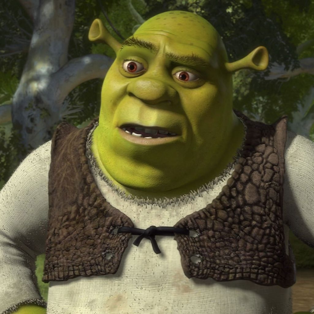
2. Human and Ogre Shrek Hybrid


3. Jasmin and Aladin and the little mermaid hybrid
This is a failed example.


4. Peace and Hare
This is a failed example, better images could have been obtained.


2.3 Gaussian & Laplacian Stacks
In this section we created and visualized the Gaussian Laplacian stacks to seamlessly blend two images using multi-resolution blending. We’ve also done a comparison of grayscale and color multi-resolution blending of generataing an Oraple image from the 1983 by Burt and Adelson(1983).
From the onset, it can be seen below that color is better than grayscale. Color helps us appreciate and see the different textures blend together to form one object in one image. Furthermore, we’ve observed that Laplacian stacks output dark images, so color in this case is better.


a)Grayscale Oraple b)Color Oraple
Below are images from the Laplacian stacks blending for creating an Oraple image. The first 3 rows shows level [4,2,0] of the Laplacian stack.The aim here was to replicate output and work done Burt and Adelson(1983) and the output from Szeliski(2020)’s textbook. The Oraple was created using a regular mask which was the same size as the images and had 0s on the right (black) and 1s on the left (white).


Level 4


Level 2


Level 0


The Oraple
2.4 Multi-resolution Blending
As a continuation from the previous section, in this section we implemented Multi-resolution Blending on other images different from the above Oraple example.
Multi-resolution Blending of the Mona Lisa Painting
This is a multi-resolution blending of the famous Mona Lisa painting with a homemade recreated photo to portray the famous painting. This painting was recreated by a follower of the instagram account @tussenkunstenquarantaine. A regular mask with 0s (black) on top and 1s(white) at the bottom was used.
The following parameters were used to perform multiresolution blending of the image below:
- Gaussian stack: {\(ksize =20,levels =50, sigma =5\)}
- Laplacian stack :{\(ksize =20 ,levels =50, sigma =5\)}


a)Monisa Lisa Painting b)Recreated Mona Lisa Photo, c)Blended Image
Multi-resolution Blending of the Van Gogh Painting
This is a multi-resolution blending of the famous Van Gogh painting art work with a recreated hyperrealistic portrait of the famous work that almost look like photographs. The recreated hyperrealistic portrait was made by Joongwon Jeong(@joongwonjeon -instagram handle). An irregular mask shown below was used to blend the two images together. The recreated portrait is more expressive around the eyes and in the attempt to add visible emotion onto the Van Gogh painting, the images were blended around that area.
The following parameters were used to perform multi-resolution blending of the image below:
- Gaussian stack: {\(ksize =20,levels =30, sigma =5\)}
- Laplacian stack :{\(ksize =20 ,levels =30, sigma =5\)}


) Van Gogh Painting b)Recreated Van Gogh Photo, c)Blended Image

Irregular Mask
3 Conclusion
This assignment was very interesting and I got to learn new things. The coolest thing I learnt in this assignment is the concept of hybrid images. I find it very cool that two images can be made into one and based on your distance you’ll be able to see the either the low frequency image or high frequency image.
4 References
Burt, P.J. and Adelson, E.H. (1983). A multiresolution spline with application to image mosaics. ACM Transactions on Graphics (TOG), 2(4), pp.217–236.
Efros, A. and Kanazawa, A. (2021). Convolution and Image Derivatives. [online] Available at: https://inst.eecs.berkeley.edu//~cs194-26/fa21/Lectures/ConvolutionAndDerivatives.pdf [Accessed 22 Sep. 2021].
Efros, A. and Kanazawa, A. (2021). Pyramid Blending, Templates, NL Filters. [online] Available at: https://inst.eecs.berkeley.edu//~cs194-26/fa21/Lectures/PyramidsBlending.pdf [Accessed 22 Sep. 2021]
Szeliski, R. (2020). COMPUTER VISION : algorithms and applications. S.L.: Springer Nature.
5 Acknowledment
None of the images I used in this assignment belong to me. Here are the sources for the images.
- Camera man:https://inst.eecs.berkeley.edu/~cs194-26/fa20/hw/proj2/cameraman.png
- Fox:https://i.pinimg.com/originals/d6/e5/83/d6e5834c67b1017265cde39ed23e7431.jpg
- Lion’s Head, Cape Town : https://goldwallpapers.com/uploads/posts/outdoor-desktop-wallpaper/outdoor_desktop_wallpaper_027.jpg
- Rhinos :https://www.hd-freewallpapers.com/latest-wallpapers/wild-animals-photo-gallery-download.jpg
- Winelands: https://content.presspage.com/uploads/685/1920_franschhoeksouthafrica-9.jpg?10000
- Eagle: https://i.pinimg.com/originals/d0/55/fc/d055fc007975005e02136140f0eaf9ab.jpg
- Orge Shrek: https://pyxis.nymag.com/v1/imgs/395/d2e/ba33266c2d32a06f263acb12d378f7b656-06-shrek.rsquare.w1200.jpg
- Peace sign: https://www.istockphoto.com/photo/hand-gesturing-peace-gm936587386-256224432
- Hare - https://thereaderwiki.com/en/Hare
- Recreated Mona lisa : https://www.instagram.com/tussenkunstenquarantaine/
- Recreated Van Gogh : https://www.instagram.com/joongwonjeong/