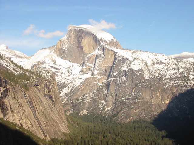
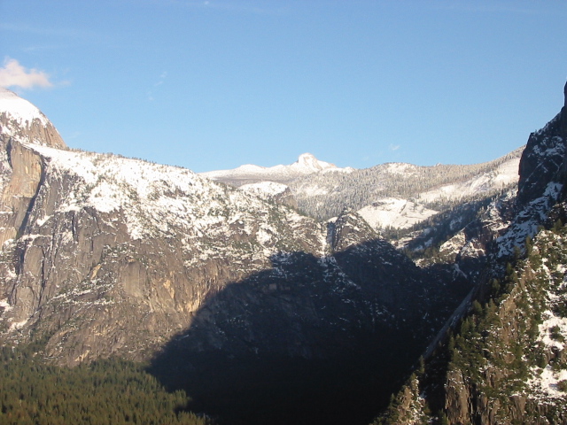
Shoot the Pictures
We obtained some pictures from the website of this class.
| Left | Right |
|---|---|
 |  |
 |  |
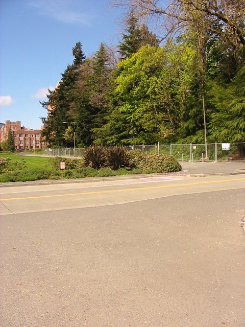 | 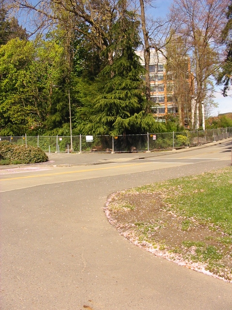 |
Recover Homographies
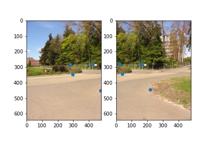
For each pair of pictures, we manually defined at least 4 pairs of corresponding points, shown below in blue dots.
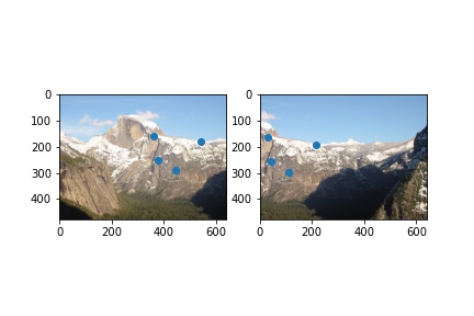
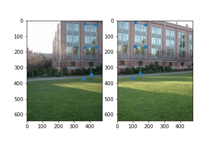
Given the points, we could construct an overdetermined system of linear equations and solve for the coefficients in the homography matrix with least squares using the equation below (taken from here).

Warp the Images
Given the original image and a homography matrix, we could obtain the transformed image using the method from project 3. We first compute the maximum and minimum coordinates of the transformed image by applying the transformation to the 4 corners. We use the transformed coordinates of the corners to obtain the size of the new image. For each pixel in the new image, we apply the inverse homography transformation to its coordinates to get the source coordinates from the original image. Finally, we use bilinear sampling to obtain the colors of each transformed pixel.
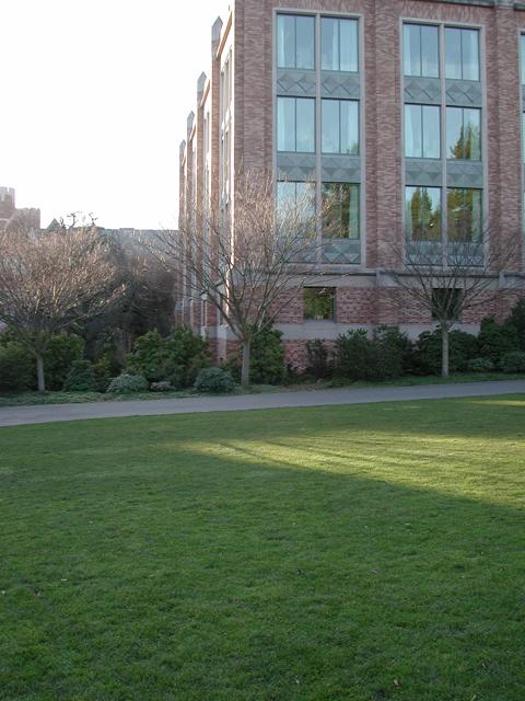
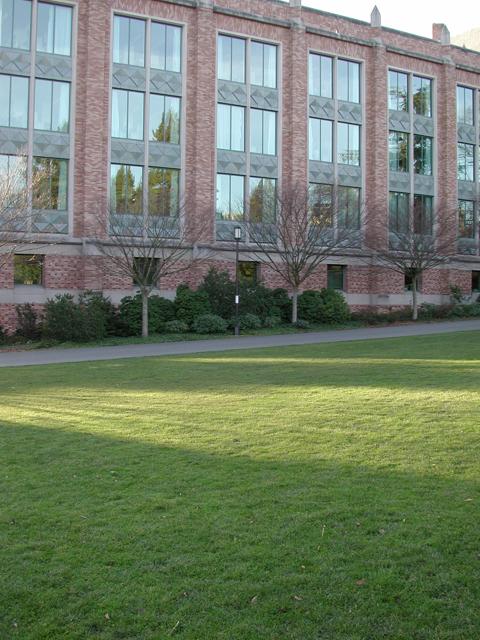
Image Rectification
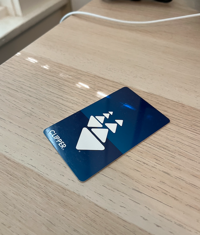
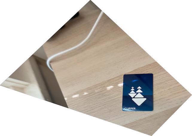
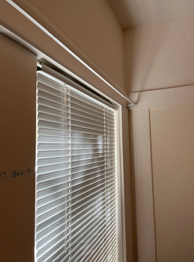
To test that the image warping works, we applied the transformation by rectifying the rectangular surfaces in some images. The card in the first image is transformed to some inner rectangle of the target image. The window in the second image is transformed to the corners of the target image similar to the transformation performed when scanning documents with phone cameras.
| Original | Rectified |
|---|---|
 |  |
 | 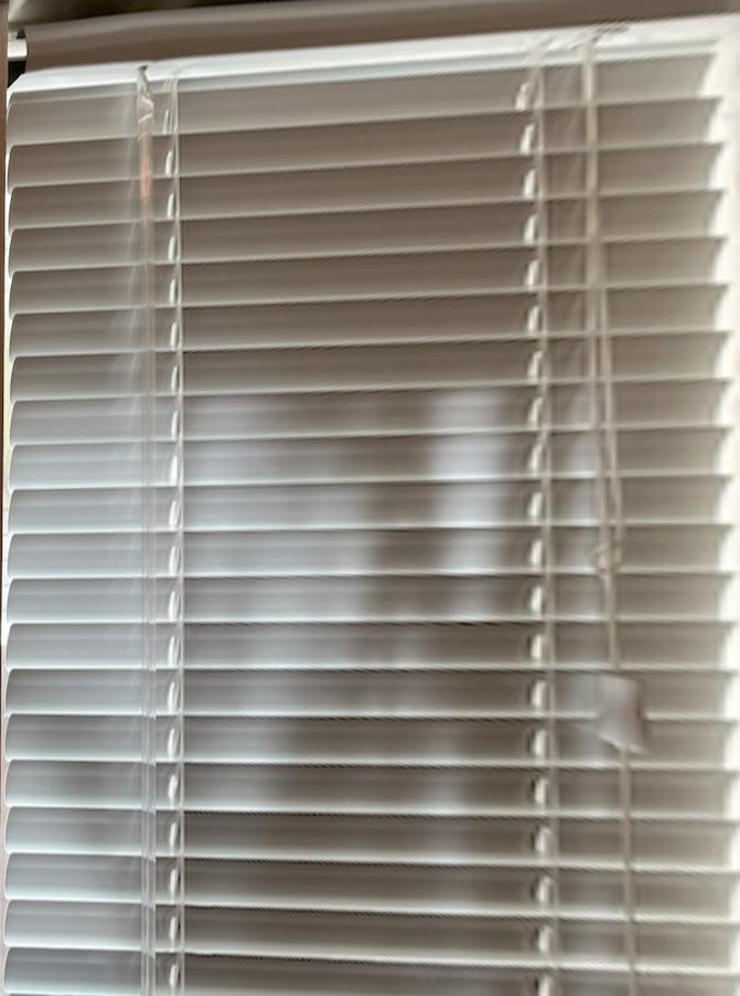 |
Blend the Images into a Mosaic
We first warped the images using the homographies recovered with the corresponding points defined in the previus parts. We then applied alpha blending on the images to compute the colors in the overlapping parts to obtain the final image. (We used the distances from the center of the image to compute the alpha values.)
| Mosaics |
|---|
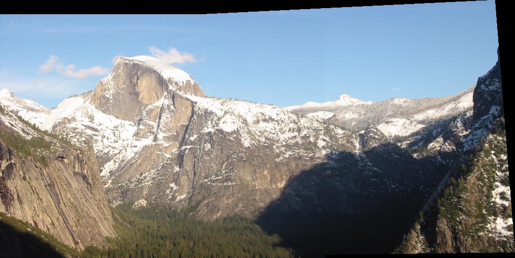 |
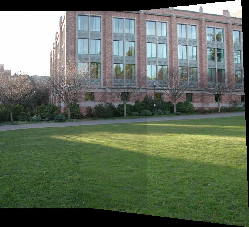 |
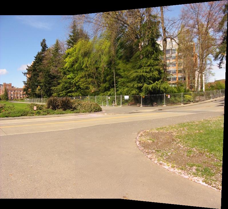 |
Tell us what you’ve learned
Seeing the application of homography matrices in action and learning the mechanics behind document scanning is pretty interesting!