|
|
|
|
|
|
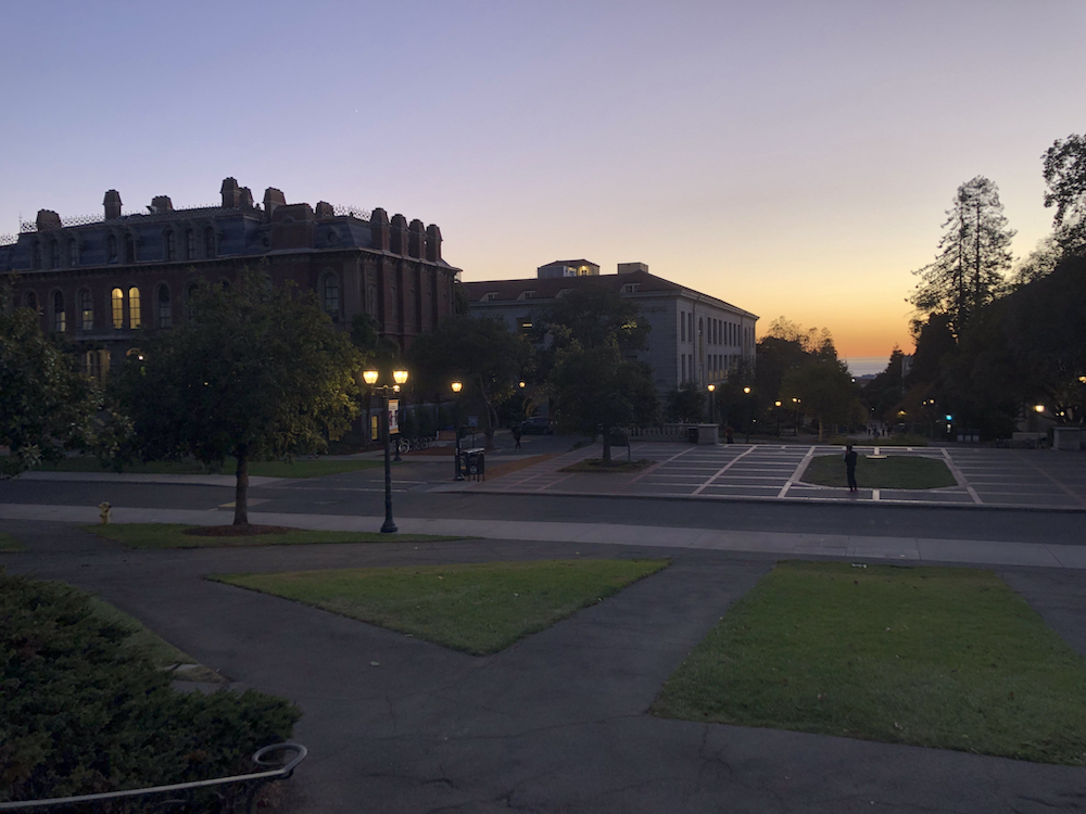
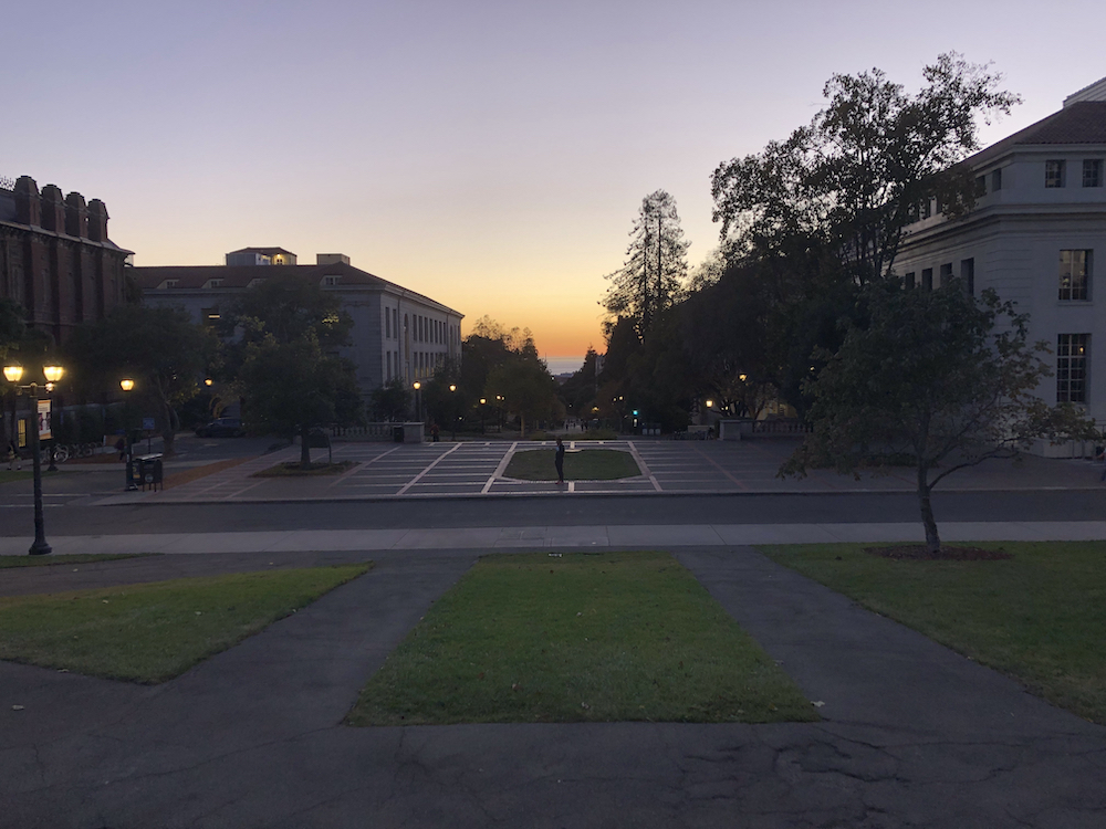
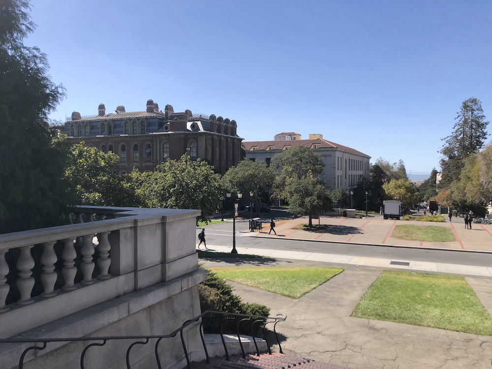
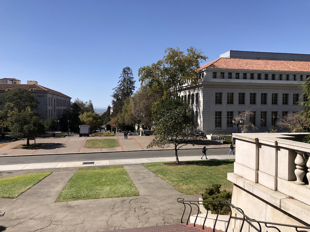
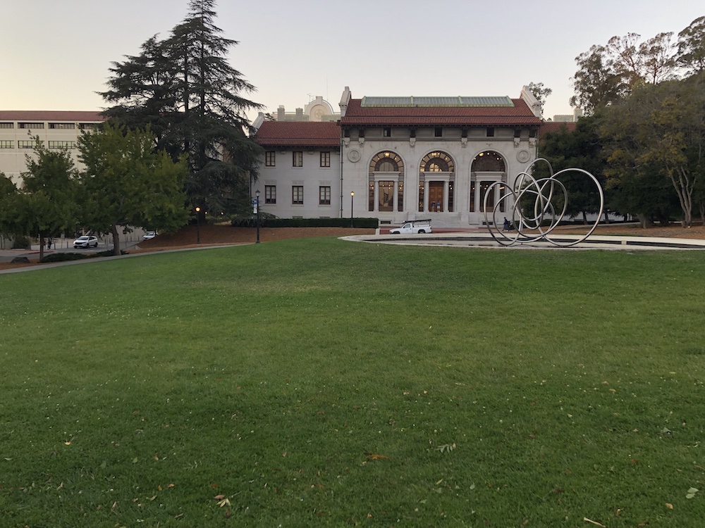
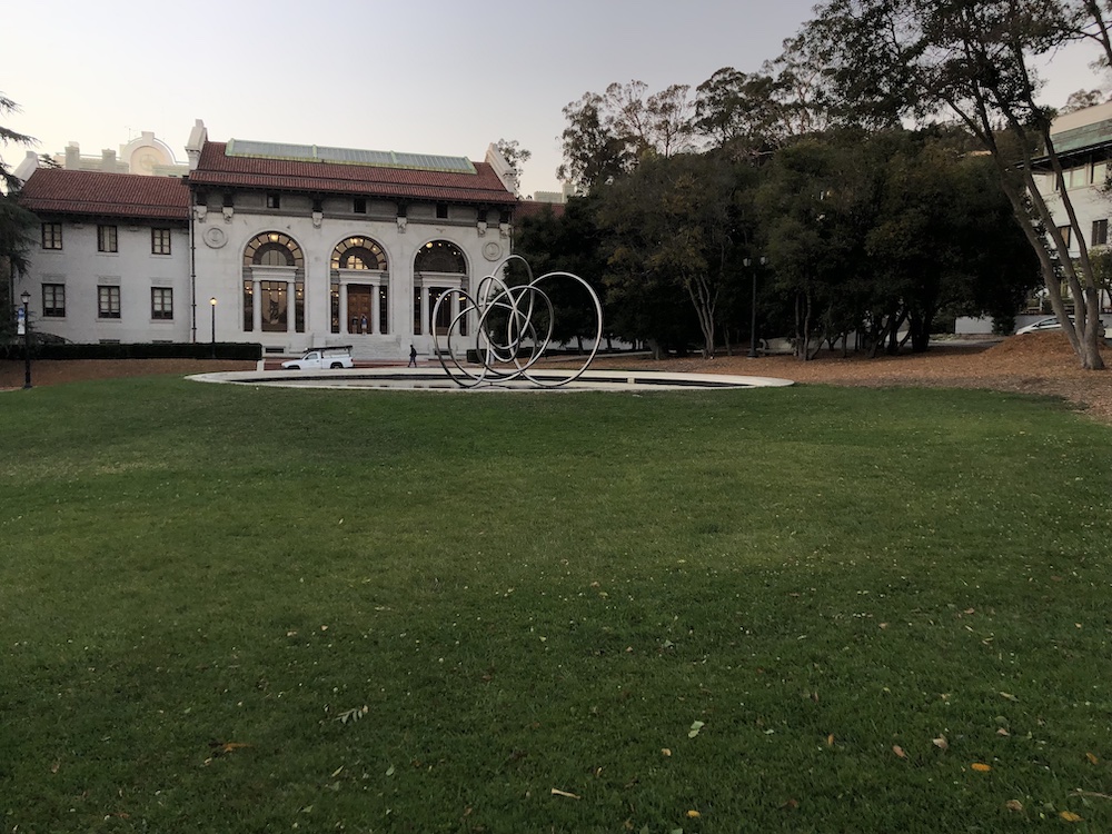
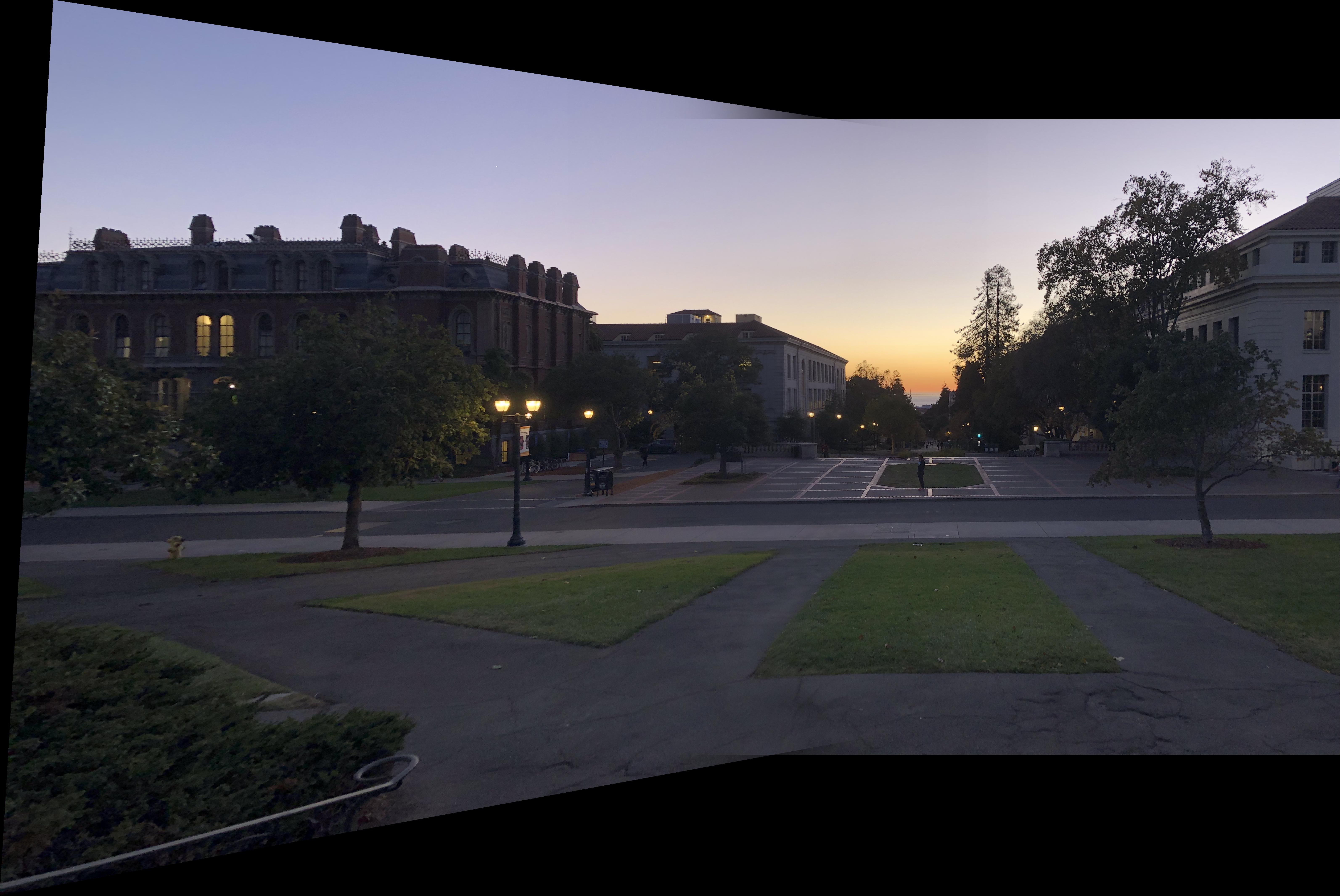
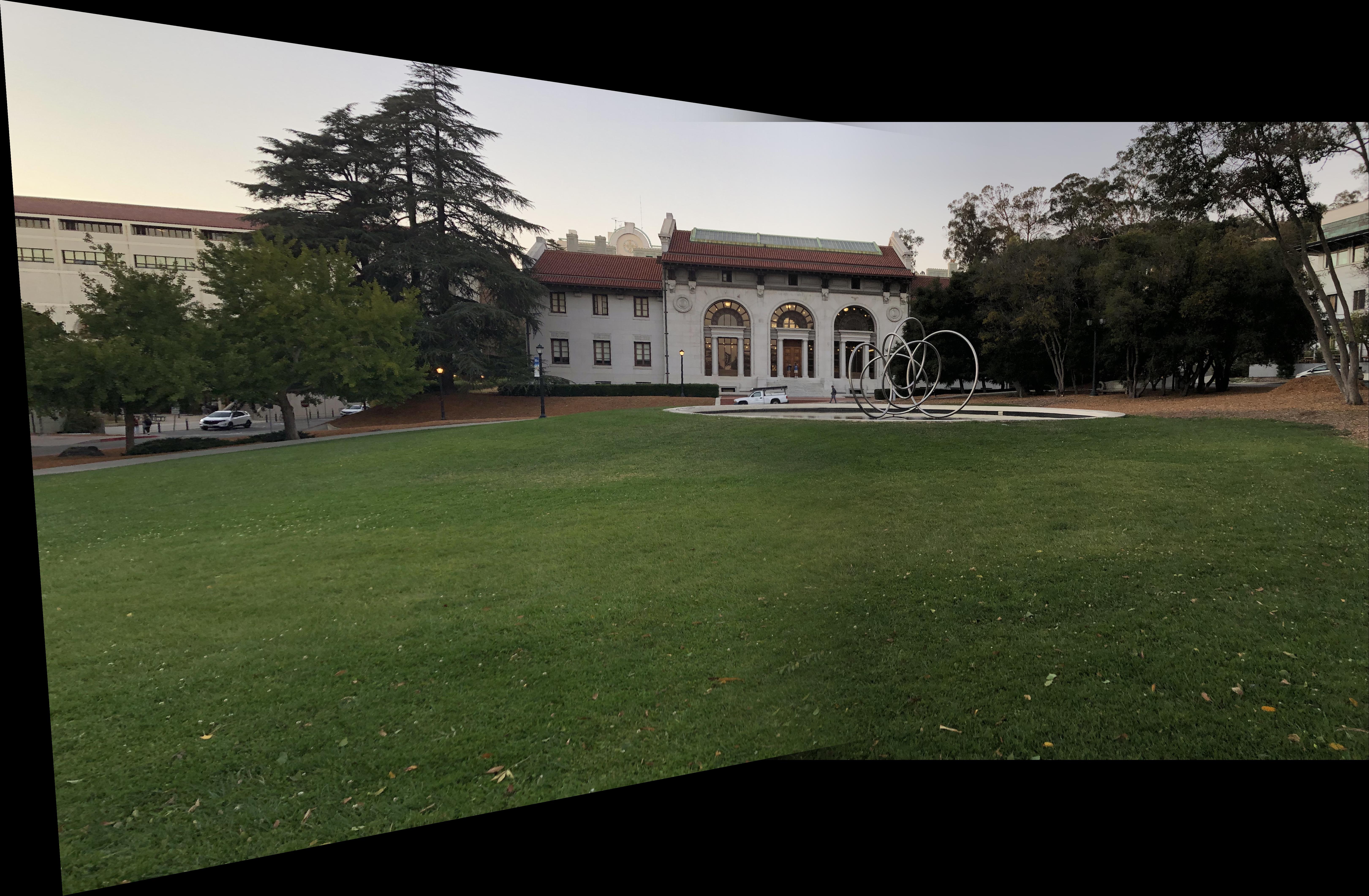
To contextualize the rest of this paper, I captured the following images when doing part A, and use them for this part as well.
|
|
|
|
|
|
|
|
|
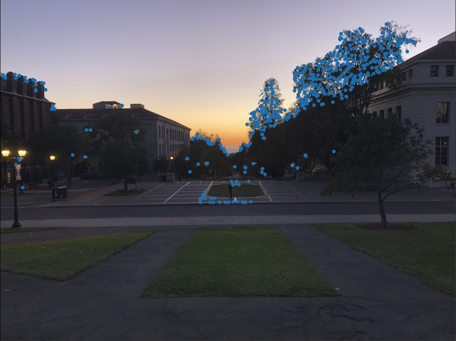
To begin, we want to gather all relevant corners in the image, regardless of rotation. To do so, we use the Harris detector due to its rotation invariance and partial invariance to affine intensity changes. After this, we have a multitude of corner points on the image, as highlighted below.
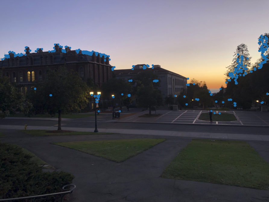
Way Dusk - Left |
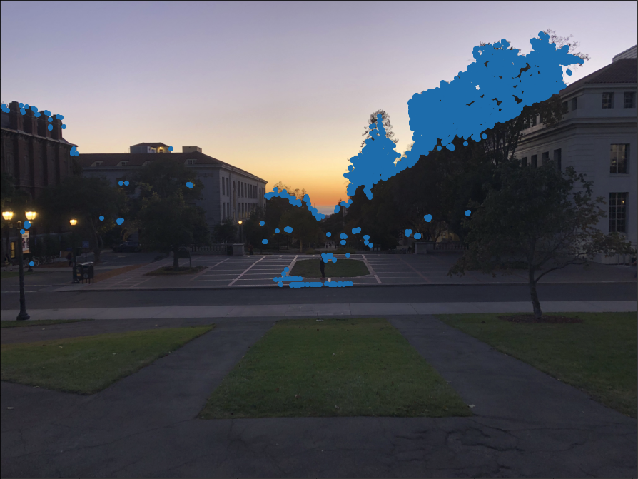
Way Dusk - Center |
In order to reduce the computation time to a practical level, we use Adaptive Non-Maximal Suppression (ANMS) to filter out a fixed number of the most optimal corner points. More specifically, in ANMS, I choose the 500 coners that are the most spatially distributed (have the furthest minimum distance to) the other Harris corners of greater intensity. With ANMS, the corners above are filtered out to the following corners below.

Way Dusk - Left |
Way Dusk - Center |
Note: the ANMS corners for the left image look similar in quantity to the original Harris corners for that image because there were 511 Harris corners gathered there, so only 11 points (which are mostly unnoticeable on the image) were filtered out.
With our cut-down set of corners from each image, we can now extract a feature descriptor for each corner. To do so, we gather axis-aligned patches from the image around each corner point. These patches are 40x40 in the raw image, and are then bias-variance normalized and scaled down to 8x8 patches. These are the final features we will use for matching corners in the next section.
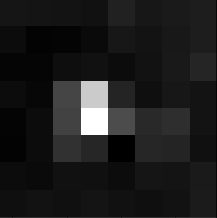
Way Dusk - Left |
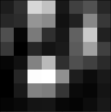
Way Dusk - Center |
To find the best feature matches between the two images we apply nearest neighbors. For each patch, I iterate through all possible patches in the other image and compute the nearest neighbor and second-nearest neighbor based on the Sum-Squared Distances (SSD) between the original patch and the other patch. Then, similar to Lowe's thresholding, I check if 1 - the ratio of the 1-NN SSD to the 2-NN SSD is greater than a threshold (I chose 0.5). If it is, then the patch and its nearest neighbor are a match. If not, then the patch has no match and will be ignored for subsequent steps. The corner points with matches are highlighted below in blue (versus the original set of corners from ANMS in red).
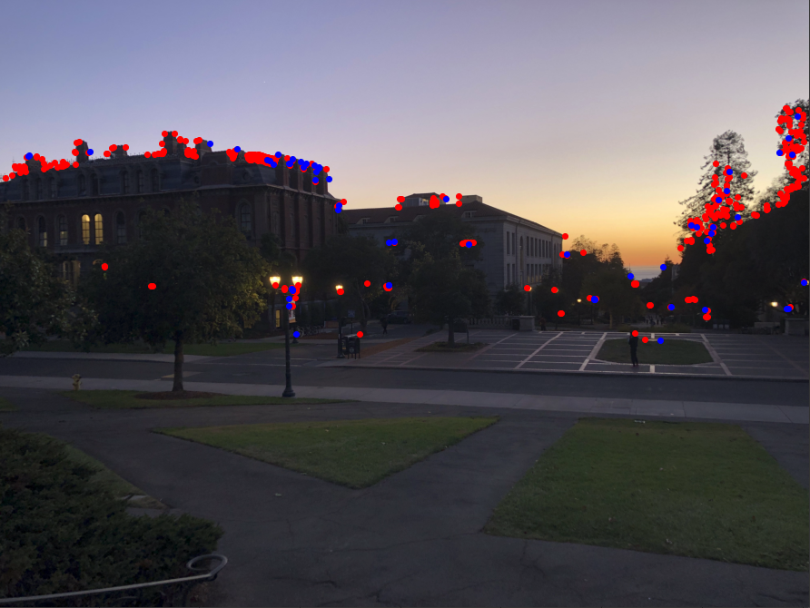
Way Dusk - Left |
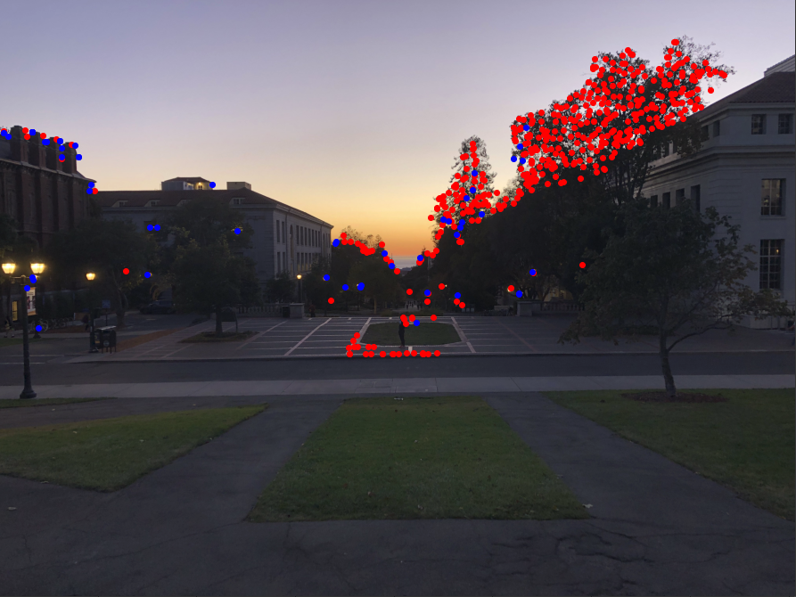
Way Dusk - Center |
With the pairs of corners, we need to finally select which corners can best help us approximate the perspective transformation between the images. To do so, we use the RANSAC method to gather the best homography between the two images. This involves using a random selection of 4 point pairs to compute an exact homography matrix and gathering the inliers (which are the point pairs that are accurately represented by the homography, up to an SSD of 0.5 in my implementation). I repeat this randomized process 5000 times and take the least-squares estimate of the homography matrix based on the largest set of inliers achieved in the randomized loop, and that homography matrix is the final homography used for the image stitching. The final RANSAC inliers are highlighted below in yellow (versus the original set of corners from ANMS in red).

Way Dusk - Left |
Way Dusk - Center |
Note the yellow points are hard to see in the original page but opening the image in a new tab will make it easier to zoom in and discern the points.
With the final homography matrix, we have all the information we need to stitch the images together. Using my image warp and blending code from Project 4A (linked above), I warp the images together with the RANSAC homography matrix to ge the final stitched image below.
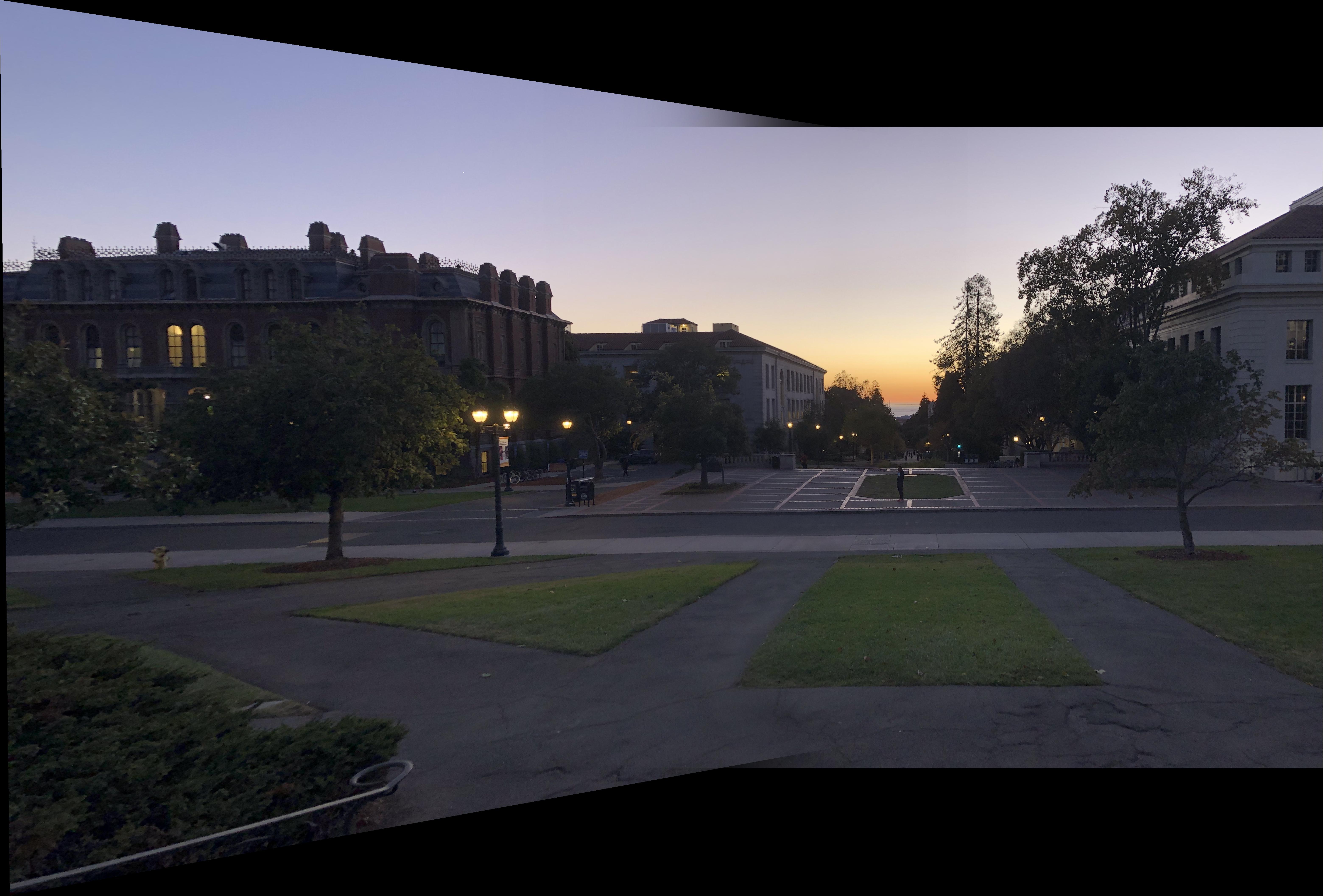
Way Dusk - Left & center |
Center Merged Manually |
Center Merged Automatically |
|
|
|
|
|
|
I learned a lot about automatic image processing for feature point detection from this project. I was very used to thinking that detecting similarities in an image was very context-heavy, requiring some level of machine learning to be able to find similarities and correspondence points automatically. With this project, however, I got to see how accurate you could be without needing anything more than pixel comparisons and RANSAC. I was also surprised by the power of the 1-NN and 2-NN thresholding to find valid correspondence points that actually matched based on some simple feature patches. Overall, this project was super interesting to explore, and I think the coolest thing I learned was the power of simple pixel processing with a bit of computer vision and algorithmic thinking.