CS294-26 Project 4 Image Warping and Mosaicing

Jimmy Xu

Overview

The goal of the first part of the project is to explore the magic of homography via two of its applications: image rectification and image mosaicing. The goal of the second part is to automate this process via feature detector, feature descriptor, and feature matching.

Shoot and Digitize Pictures

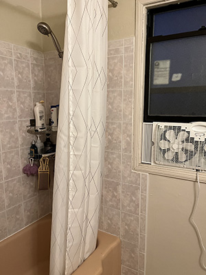
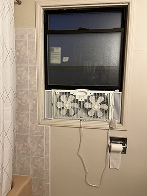
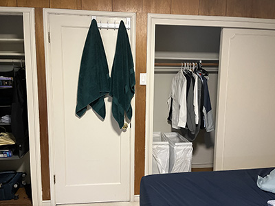
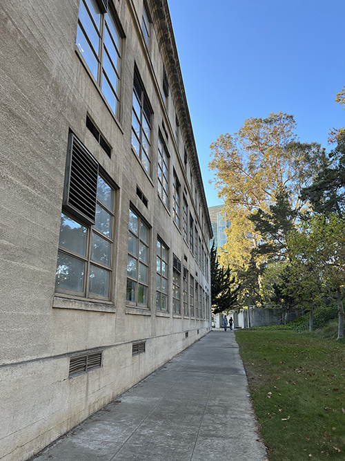
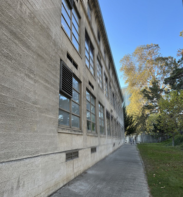
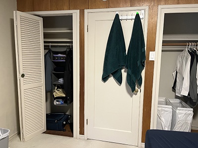
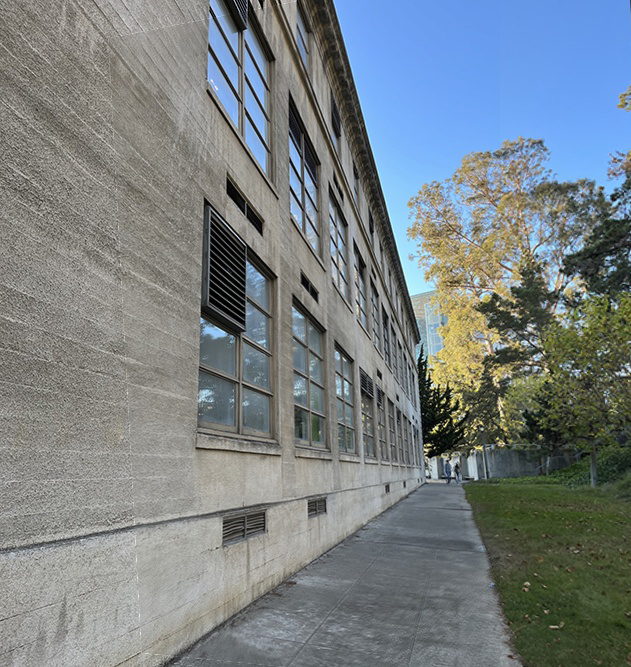
The first step is to take some pictures with the same center of projection (i.e. rotating, but not translating, the camera).

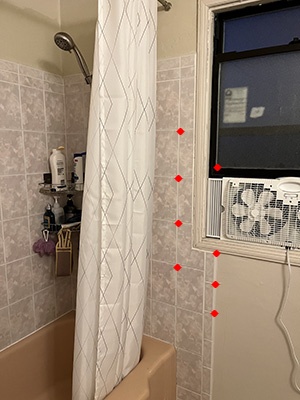
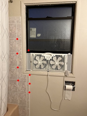
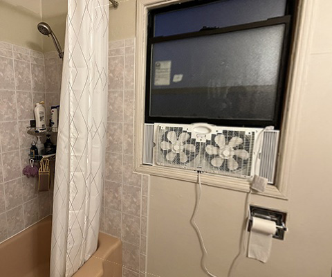
Bathroom

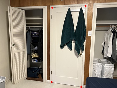
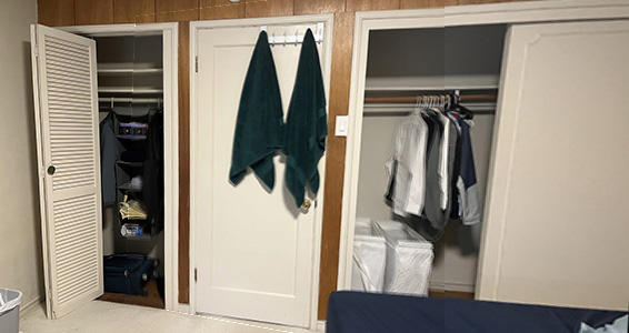
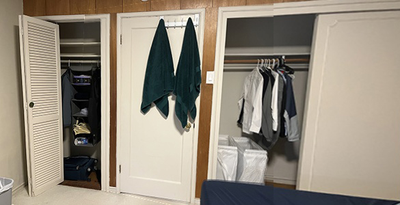
Bedroom

Lewis Hall

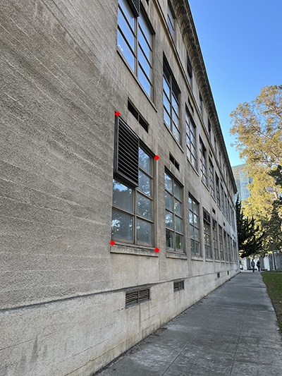
Recover Homographies

$H$ . We need at least 4 points.

By definition, perspective projection can be expressed as follows.

\begin{matrix} [\begin{array}{l} x_{a} \\ y_{a} \\ z_{a} \end{array}] = H_{3 \times 3} [\begin{matrix} x_{1} \\ y_{1} \\ 1 \end{matrix}], [\begin{matrix} \hat{x_{1}} \\ \hat{y_{1}} \\ 1 \end{matrix}] = \frac{1}{z_{a}} [\begin{array}{l} x_{a} \\ y_{a} \\ z_{a} \end{array}] \Rightarrow [\begin{matrix} {\hat{x}}_{i} z_{a} \\ {\hat{y}}_{i} z_{a} \\ z_{a} \end{matrix}] = [\begin{array}{lll} h_{11} & h_{12} & h_{13} \\ h_{21} & h_{22} & h_{23} \\ h_{31} & h_{32} & h_{33} \end{array}] [\begin{matrix} x_{i} \\ y_{i} \\ 1 \end{matrix}] \end{matrix}

$H$ . Following this pattern, we can add more points to the giant matrix on the left.

\begin{matrix} [\begin{array}{cccccccc} x_{1} & y_{1} & 1 & 0 & 0 & 0 & - x_{1} {\hat{x}}_{1} & - y_{1} \hat{x_{1}} \\ x_{2} & y_{2} & 1 & 0 & 0 & 0 & - x_{2} \hat{x_{2}} & - y_{2} \hat{x_{2}} \\ x_{3} & y_{3} & 1 & 0 & 0 & 0 & - x_{3} \hat{x_{3}} & - y_{3} \hat{x_{3}} \\ x_{4} & y_{4} & 1 & 0 & 0 & 0 & - x_{4} \hat{x_{4}} & - y_{4} \hat{x_{4}} \\ 0 & 0 & 0 & x_{1} & y_{1} & 1 & - x_{1} \hat{y_{1}} & - y_{1} \hat{y_{1}} \\ 0 & 0 & 0 & x_{2} & y_{2} & 1 & - x_{2} \hat{y_{2}} & - y_{2} \hat{y_{2}} \\ 0 & 0 & 0 & x_{3} & y_{3} & 1 & - x_{3} \hat{y_{3}} & - y_{3} \hat{y_{3}} \\ 0 & 0 & 0 & x_{4} & y_{4} & 1 & - x_{4} \hat{y_{4}} & - y_{4} \hat{y_{4}} \end{array}] [\begin{array}{l} h_{11} \\ h_{12} \\ h_{13} \\ h_{21} \\ h_{22} \\ h_{23} \\ h_{31} \\ h_{32} \end{array}] = h_{33} [\begin{matrix} {\hat{x}}_{1} \\ \hat{x_{2}} \\ \hat{x_{3}} \\ \hat{x_{4}} \\ \hat{y_{1}} \\ \hat{y_{2}} \\ \hat{y_{3}} \\ \hat{y_{4}} \end{matrix}] where h_{33} can be set to be 1 \end{matrix}

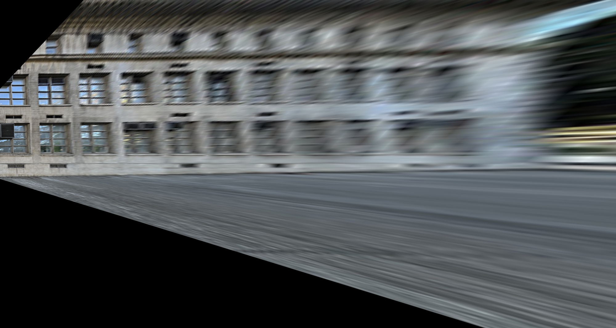
Warp the Images and Image Rectification

Once we have the homography matrix, we can warp the image. If we set the destination to be a rectangle, we can make a plane frontal-parallel. I referred to [2] for some help with cv2.remap.

We can do the same thing for a more extreme example

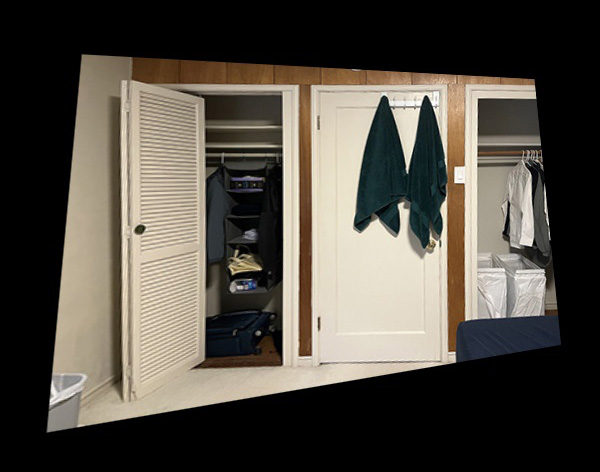
Blend the Images into A Mosaic

I can also warp one image to another and blend them, creating an image mosaic. The overlapping region of the two images are the average of them.

Feature Detector

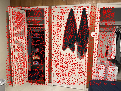
Now let's automate the process. The first step is to choose a feature detector. I used Harris Interest Point Detector. Note that the corners around the edges are filtered out.

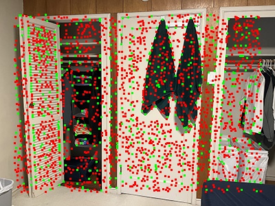
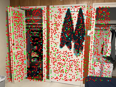
Adaptive Non-Maximal Suppression

As you can see, there are way too many corners to process efficiently. I implemented Adaptive Non-Maximal Suppression (ANMS) to spatially evenly sample features with strong corner response. I used the method described in [3]. The 500 green dots are chosen due to their relatively large radius (defined in [3]).

Feature Descriptor

The next step is to generate a scale-invariant feature descriptor. I followed the method described in [3], except the rotational invariant. For each feature, I extracted the 40x40 patch around it, downsample to 8x8, and normalize it. Here's an example.

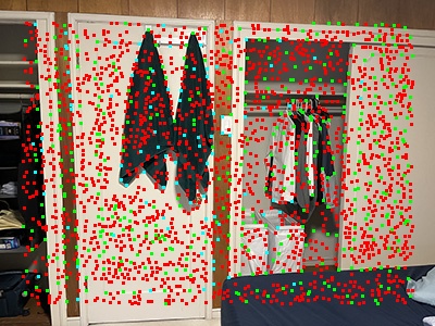
Lowe Thresholding

There are still too many features to process! I used the NN-1/NN-2 as a threshold to filter out more points, as described in [3].

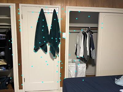Random Sample Consensus (RANSAC)

As a final step, I used the RANSAC method described in the lecture slides [4] to exclude the few outliers and compute the right homography. Here are the results.

As you can see, the RANSAC method performs better than matching via my manual labeling, especially in the last image.

Things I learned

While I think it is not too hard to grasp the idea of each step, I was still really impressed by the power of auto-stitching.

References

[1] https://towardsdatascience.com/estimating-a-homography-matrix-522c70ec4b2c

[2] https://stackoverflow.com/questions/46520123/how-do-i-use-opencvs-remap-function

[3] https://inst.eecs.berkeley.edu/~cs194-26/fa21/hw/proj4/Papers/MOPS.pdf

[4] https://inst.eecs.berkeley.edu//~cs194-26/fa21/Lectures/feature-alignment-and-flow.pdf

Manual labeling	RANSAC