Project 2: Fun with Filters and Frequencies
Project Overview
The aim of the project was to utilize different types of filters and convolution to
implement a variety of image manipuation techniques. In particular, the finite difference
filter
allowed us to detect edges within an image by visually displaying partial derivatives
in the x and y directions. Additionally, the Gaussian blur filter, despite being good at
blurring
images, was also used to sharpen images and merge two images together (in particular,
overlaying
low/high frequencies to generate a hybrid image and blending images together with the help
of
Gaussian and Laplacian stacks).
Let's explore!
Project Link
Part 1: Fun with Filters
Part 1.1: Finite Difference Operator
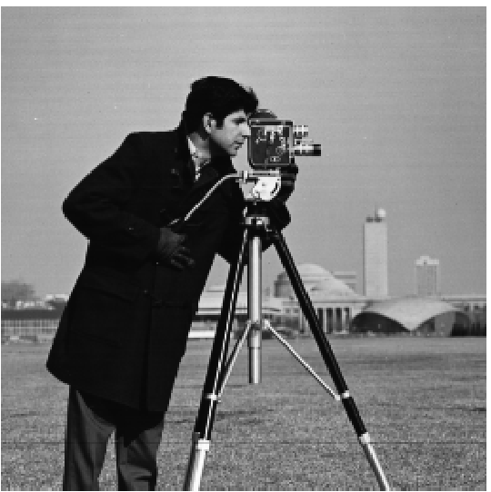
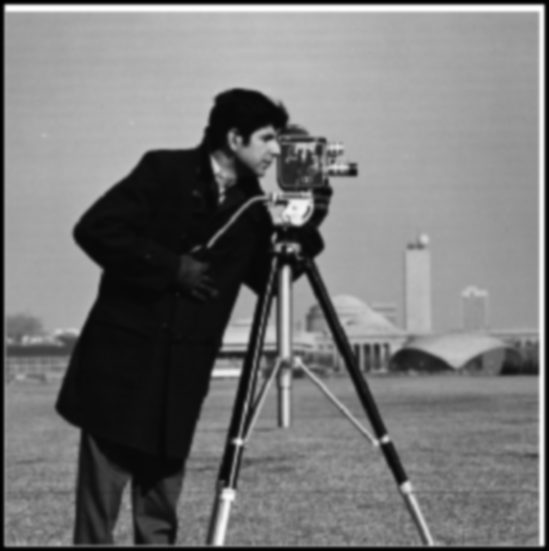
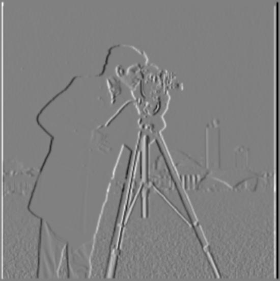
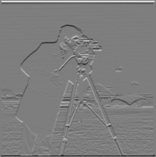
The first task was to use the finite difference operators Dx and Dy to detect horizontal and vertical edges in the cameraman image. In particular, we defined Dx = [1, -1] and Dy = [1, -1]T. Convolving these two filters with the original image would yield the horizontal and vertical edges (partial derivatives of the image in the x and y directions).
cameraman.png
Horizontal Edges (∂f/∂x)
Vertical Edges (∂f/∂y)
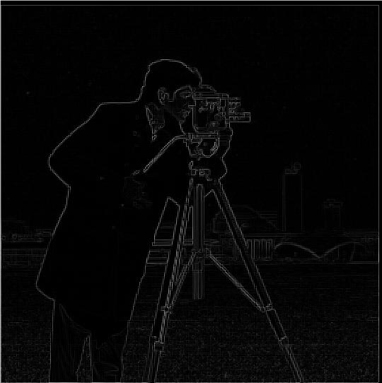
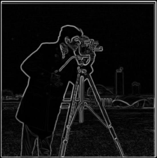
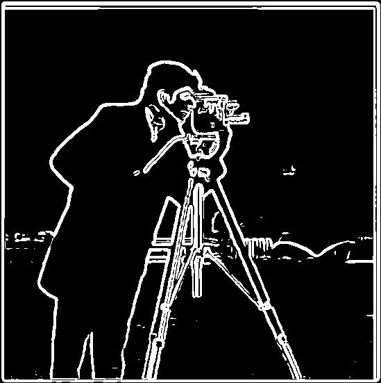
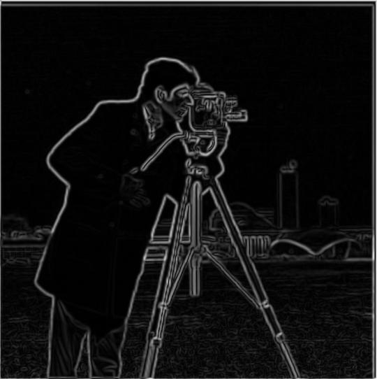
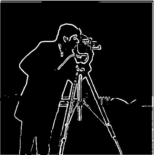
After generating both the horizontal and vertical edges, we can calculate the gradient magnitude to determine how strong the change in intensity is within the cameraman image. This is achieved by calculating sqrt((∂f/∂x)^2 + (∂f/∂y)^2) pixel-wise between the horizontal and vertical edge images (where the horizontal image is ∂f/∂x and the vertical image is ∂f/∂y). Once obtaining the gradient magnitude, we can binarize this image to show the strongest edges in the cameraman image.
Gradient Magnitude
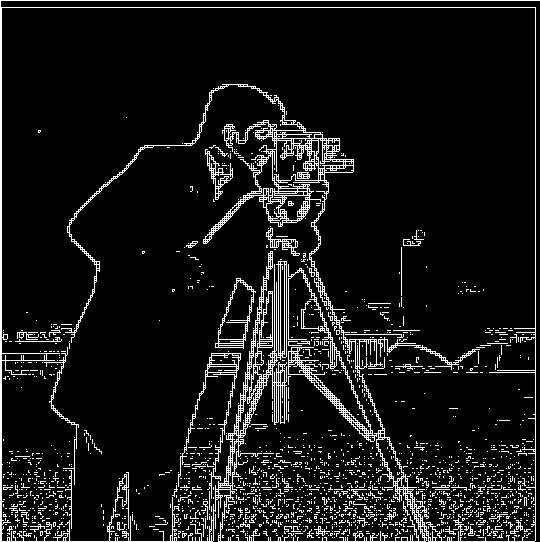
Binarized (Threshold: 0.1)
Binarized (Threshold: 0.25)
Part 1.2: Derivative of Gaussian (DoG) Filter
Notice that the binarized images are quite noisy (in other words, there are some pixels that have strong magnitude values but don't necessarily form an edge on the cameraman image). To minimize the impact of noise, we can blur the cameraman image first by convolving it with a Gaussian filter, then following the same steps as above on the blurred image. For this example, we used a Gaussian filter with a sigma of 1.5.
blurry_cameraman.png
Blurred Horizontal Edges (∂f/∂x)
Blurred Vertical Edges (∂f/∂y)

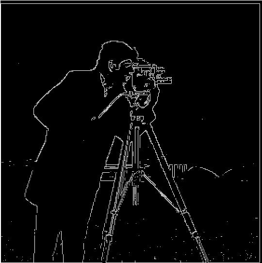
Blurred Gradient Magnitude
Binarized (Threshold: 0.05)
Binarized (Threshold: 0.08)
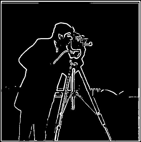
Utilizing the Gaussian filter reduced the noise that was present in the previous examples
(Part 1.1). Additionally, the edges feel much more pronounced,
as they are smoother and a bit thicker than the non-blurred counterpart.
Note that the above example required two convolutions on the cameraman image (the first by
convolving the image with the gaussian filter, and the second
by convolving the blurred image with a finite difference operator [Dx or
Dy]). Another approach is to use the derivative of gaussians:
in other words, we convolve the gaussian filter with each finite difference operators (to
get DoG(Dx) and DoG(Dy)), then convolve each
DoG filter with the original image to generate the horizontal and vertical edges. This
results in only one convolution on the cameraman image!
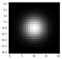
Original Gaussian (sigma: 1.5)

DoG(Dx)

DoG(Dy)

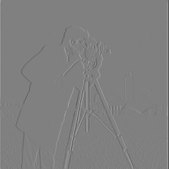
Blurred Horizontal Edges with DoG(Dx)

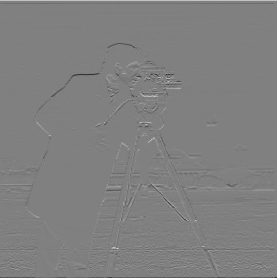
Blurred Vertical Edges with DoG(Dy)
Blurred Gradient Magnitude from DoG
Binarized (Threshold: 0.08)
Notice that our results are the same between both methods (two convolutions vs one convolution).
Part 2: Fun with Frequencies
Part 2.1: Image "Sharpening"
This task required us to sharpen images by using an "unsharp mask filter". To achieve this, we can do the following:
- 1. Blur the original image by convolving it with a Gaussian filter. This isolates the low frequencies of the image.
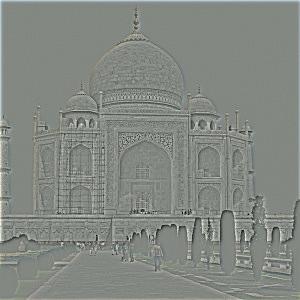
- 2. Subtract the blurred image (from 1) from the original image. This isolates the high frequencies of the image.
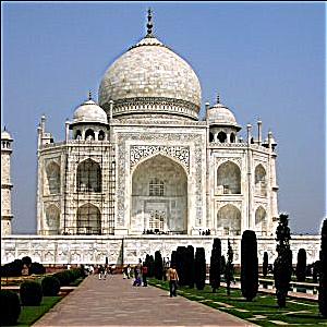
- 3. Add the high frequency image (from 2) multiplied by a factor alpha to the original image to generate a sharpened image.
We can combine the three steps into one filter:
- Given an image f we want to sharpen and a Gaussian blur filter g, our
result will be:
f + alpha * (f - convolve(f, g))
- Here, " * " represents the multiplication operation, not convolution.
- This can be simplified to: convolve(f, h), where h = (1 +
alpha) * e - alpha * g
- e is the unit impulse (matrix with same dimensions as g where every entry is 0 except a 1 at the center pixel of the filter).
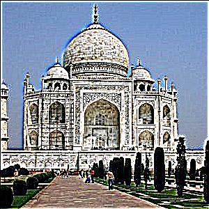
A breakdown of the sharpening process for multiple images is seen here (using a Gaussian filter with a sigma of 1.5):
taj.jpeg
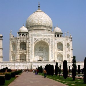
Blurred Image
Isolated High Frequencies
Final Result (alpha: 2)
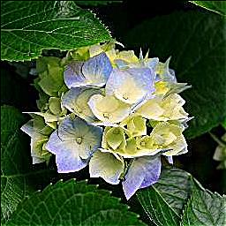
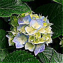
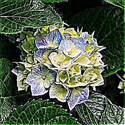
flower.jpeg

Blurred Image
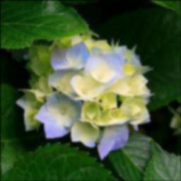
Isolated High Frequencies
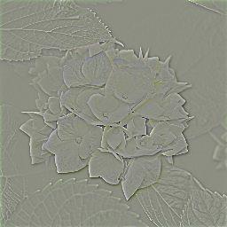
Final Result (alpha: 2)
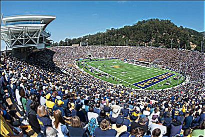
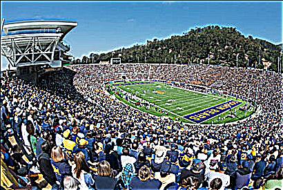
berkeley_crowd.jpeg

Blurred Image
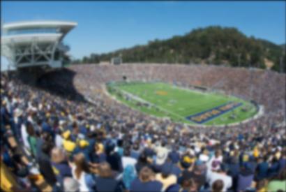
Isolated High Frequencies
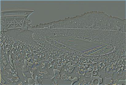
Final Result (alpha: 2)
Additionally, here's a demonstration on how changes in alpha impact the final result:
taj.jpeg
alpha: 2
alpha: 5

alpha: 10
flower.jpeg
alpha: 2
alpha: 5
alpha: 10
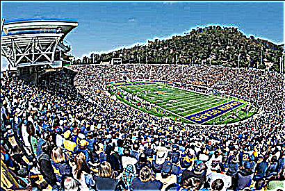
berkeley_crowd.jpeg
alpha: 2
alpha: 5
alpha: 10
Notice that this sharpening process is also fairly effective at amplifying an image that has been blurred.
doggo.jpeg
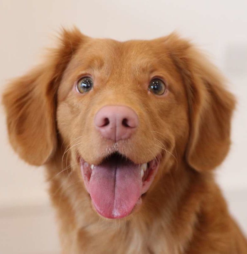
Blurred Doggo
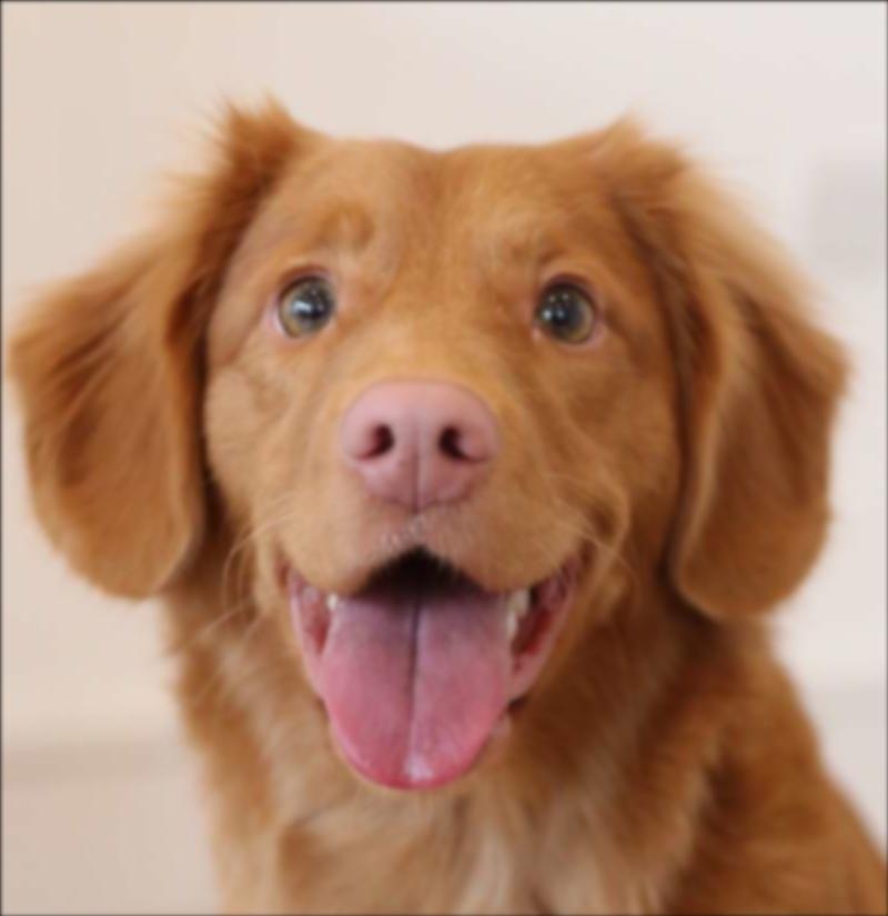
Sharpened Blurred Doggo (alpha: 2)
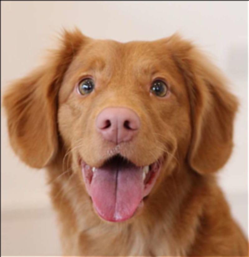
Although sharpening the blurred image does not completely recreate the original image (likely because some of the high frequencies in the original image are lost due to blurring), the unsharp mask filter does a nice job at amplifying the high frequencies to make the image appear sharper overall.
Part 2.2: Hybrid Images
This next task takes the ideas from Part 2.1 (separating images into their low and high
frequencies) and utilizes them to create hybrid images!
Specifically, hybrid images are static images that appear differently based on how closely
you view them. Specifically, high frequency attributes are
more prevalent when looking closely at an image, but low frequencies dominate when looking
at a distance. As such, we can mesh different images together
by averaging the low frequencies of one image (using a Gaussian filter) with the high
frequencies of another image (image - blurred image).
Below are examples of hybrid images, some combinations better than others.
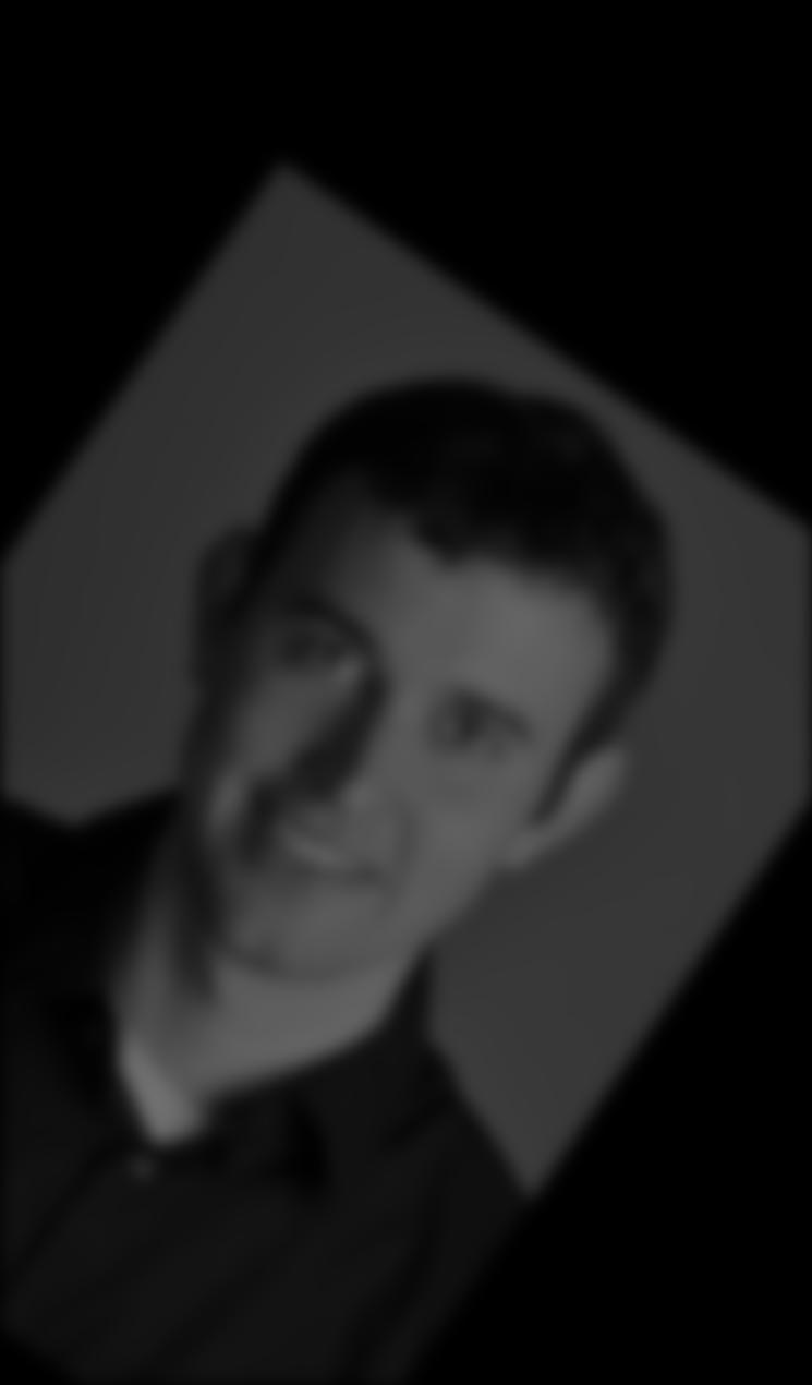
Derek/Nutmeg Combination (Class Example)
Derek
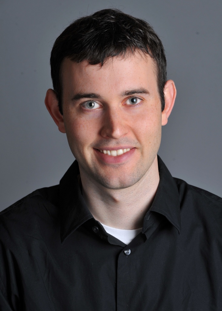
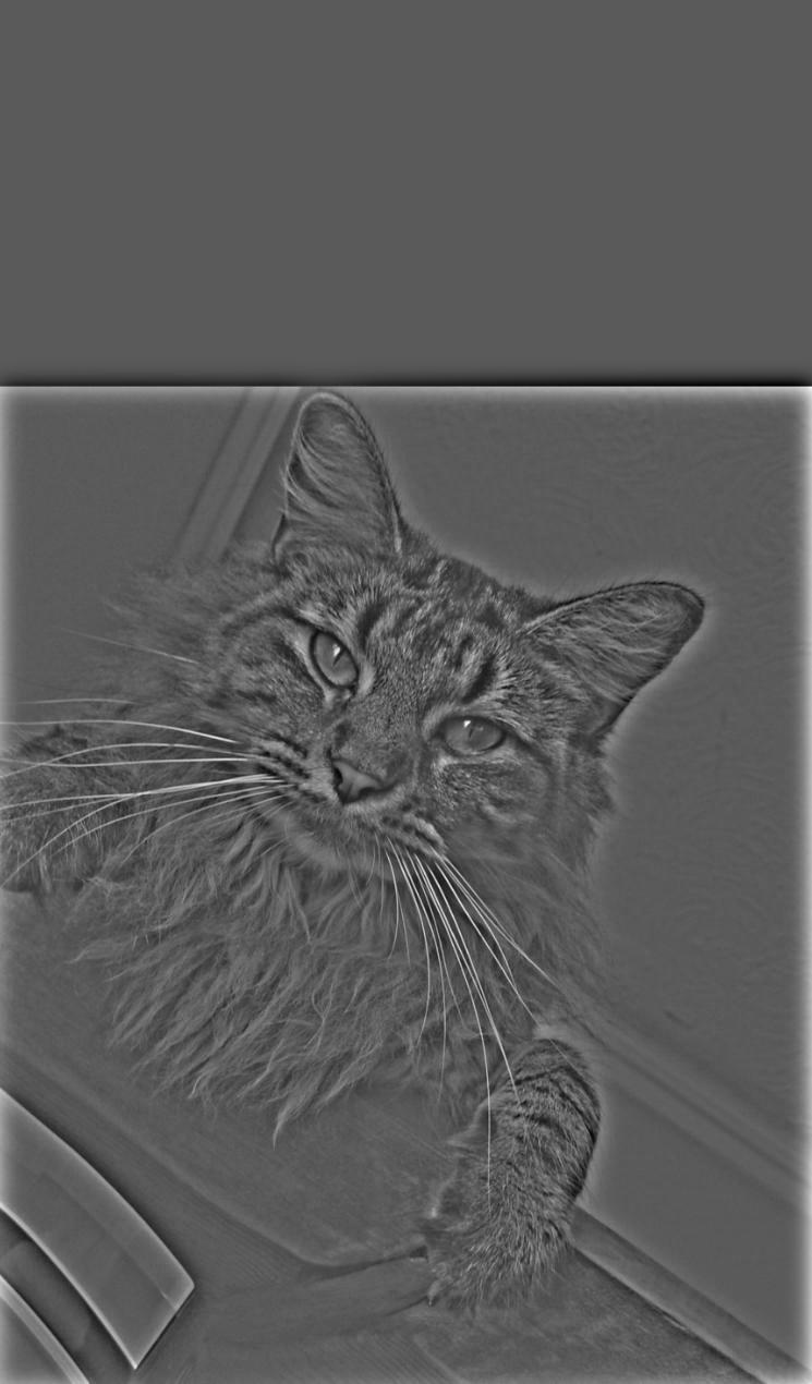
Nutmeg
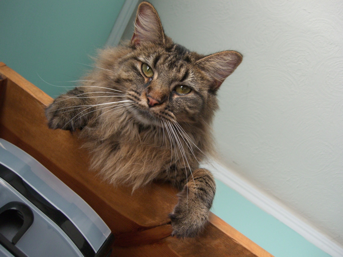
Derek (Low Frequencies)
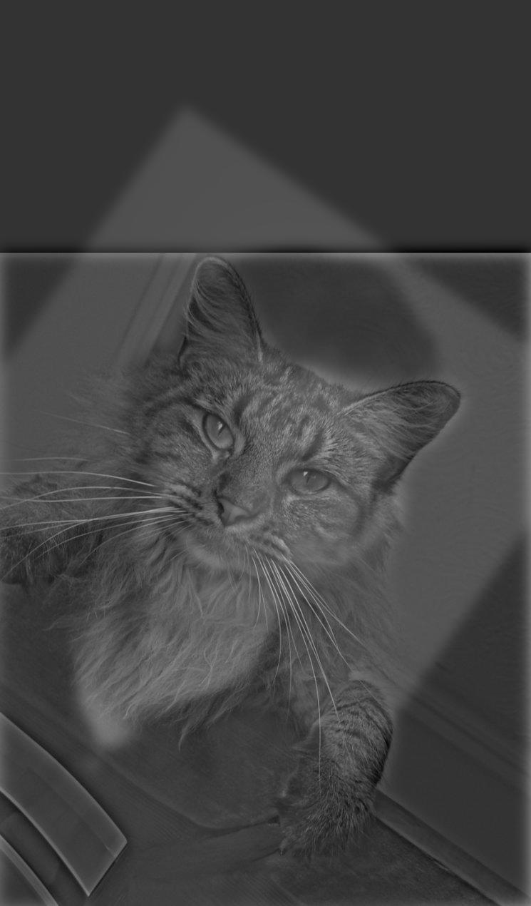
Nutmeg (High Frequencies)
Combination (Catman)
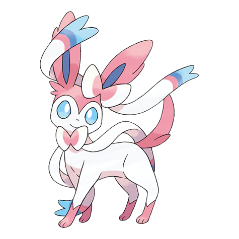
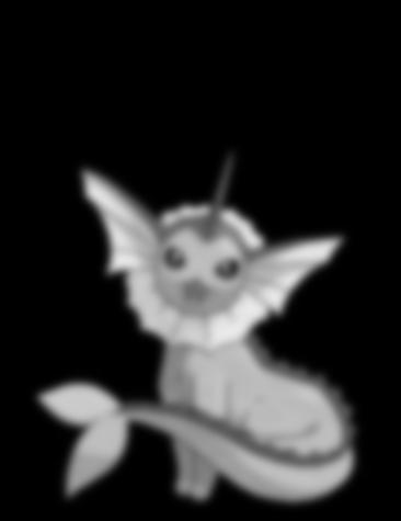
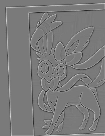
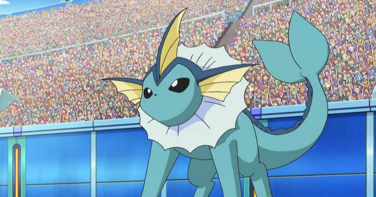
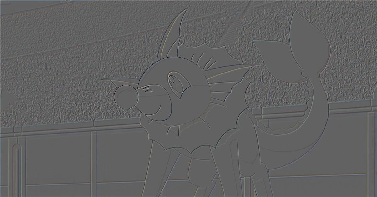
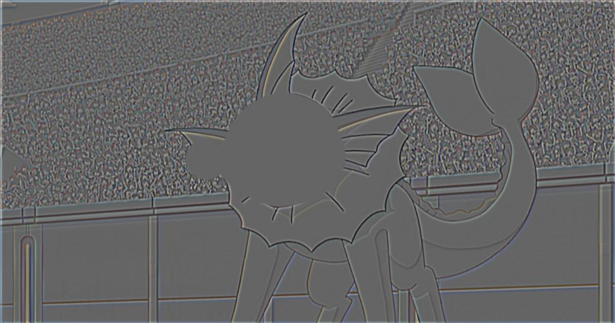
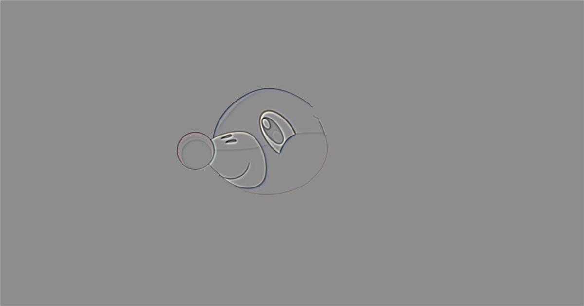
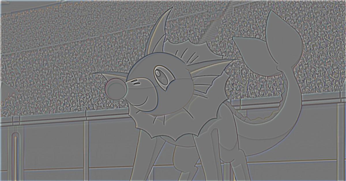
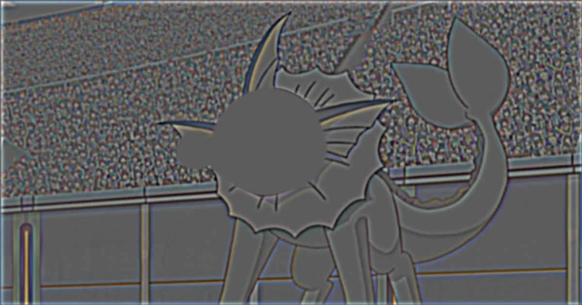
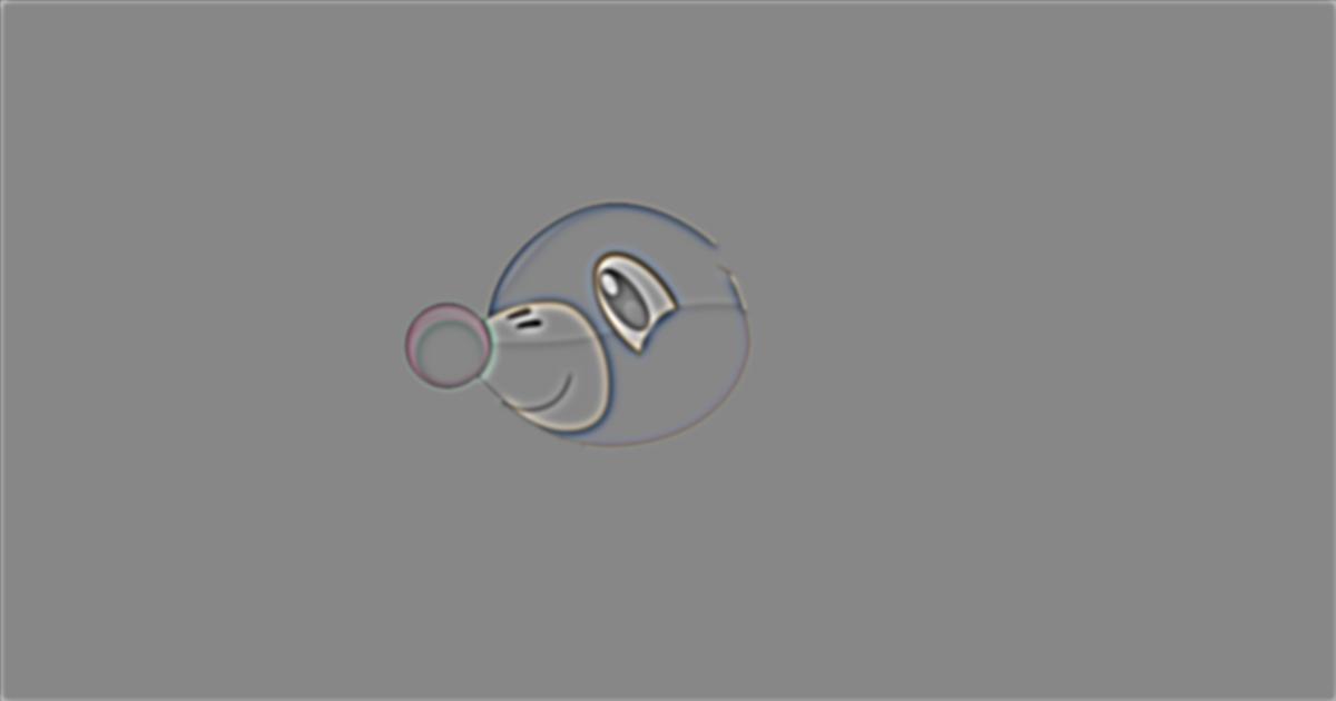
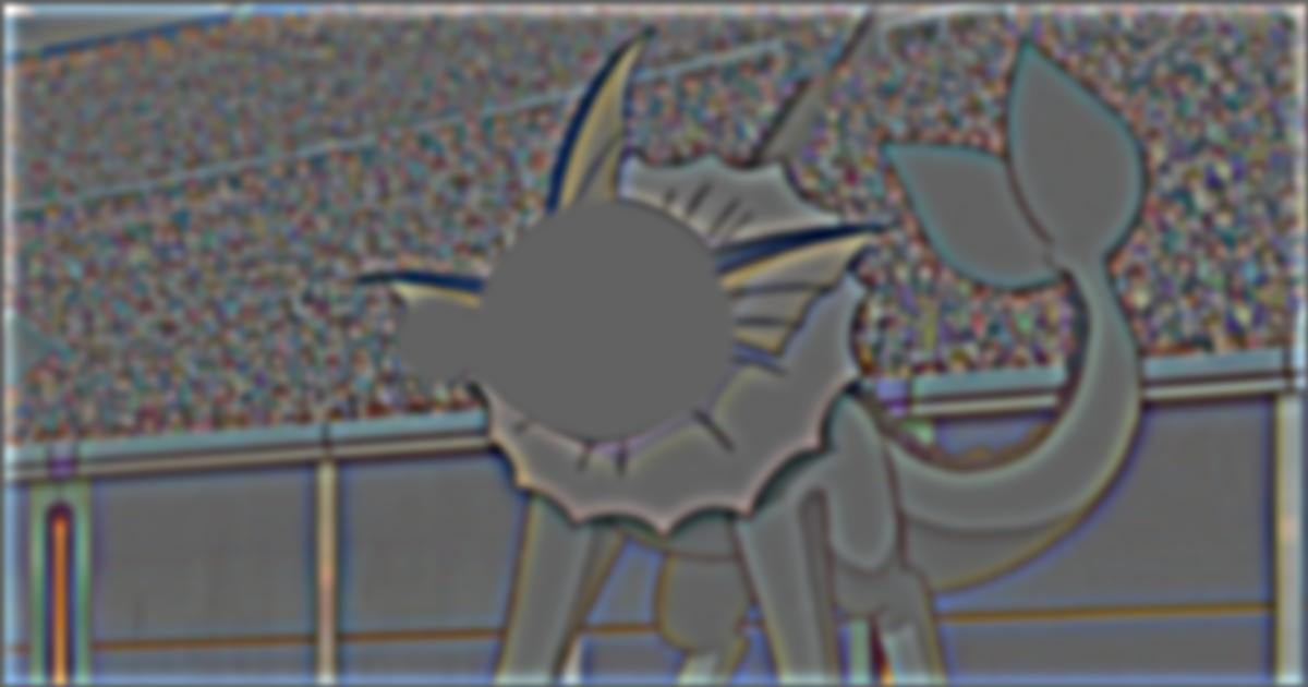
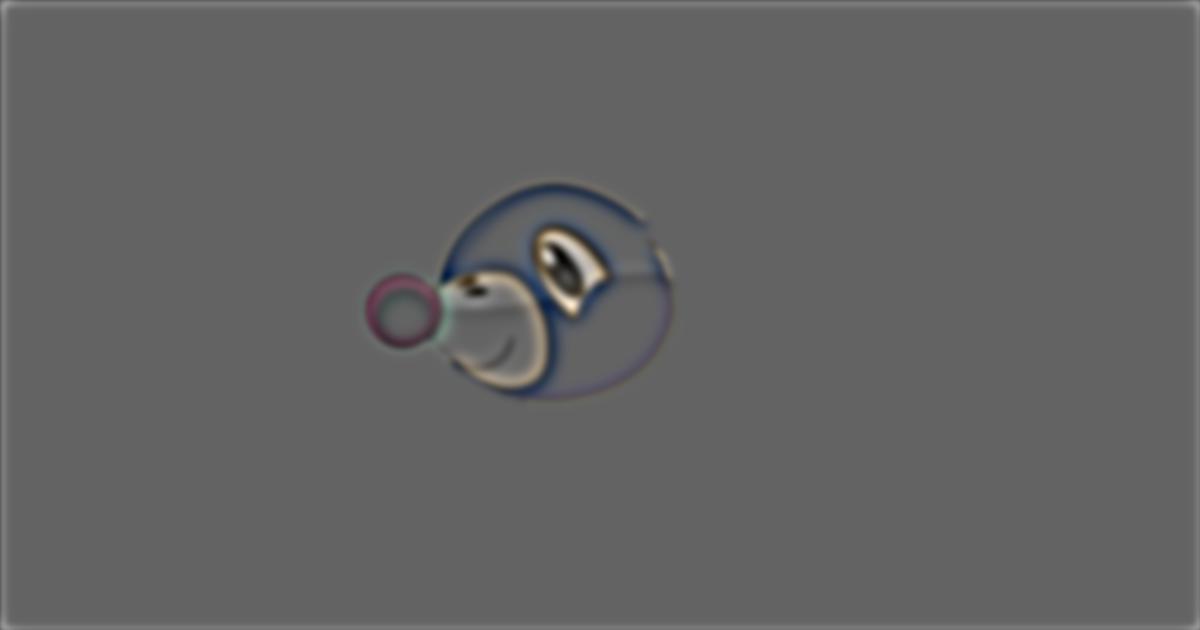
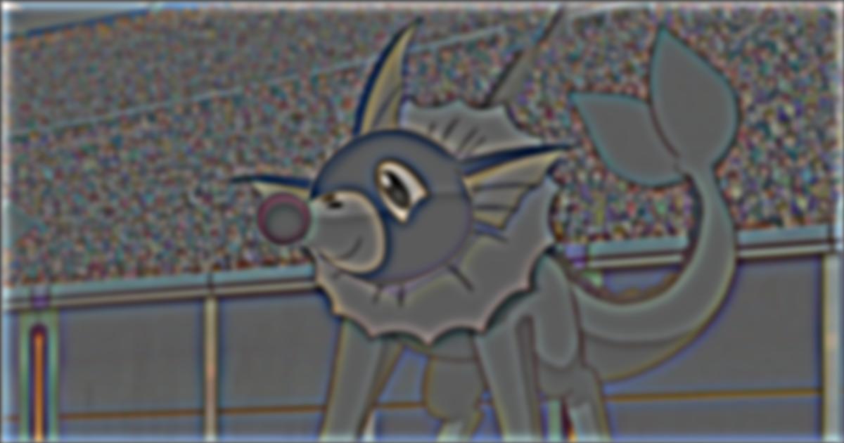
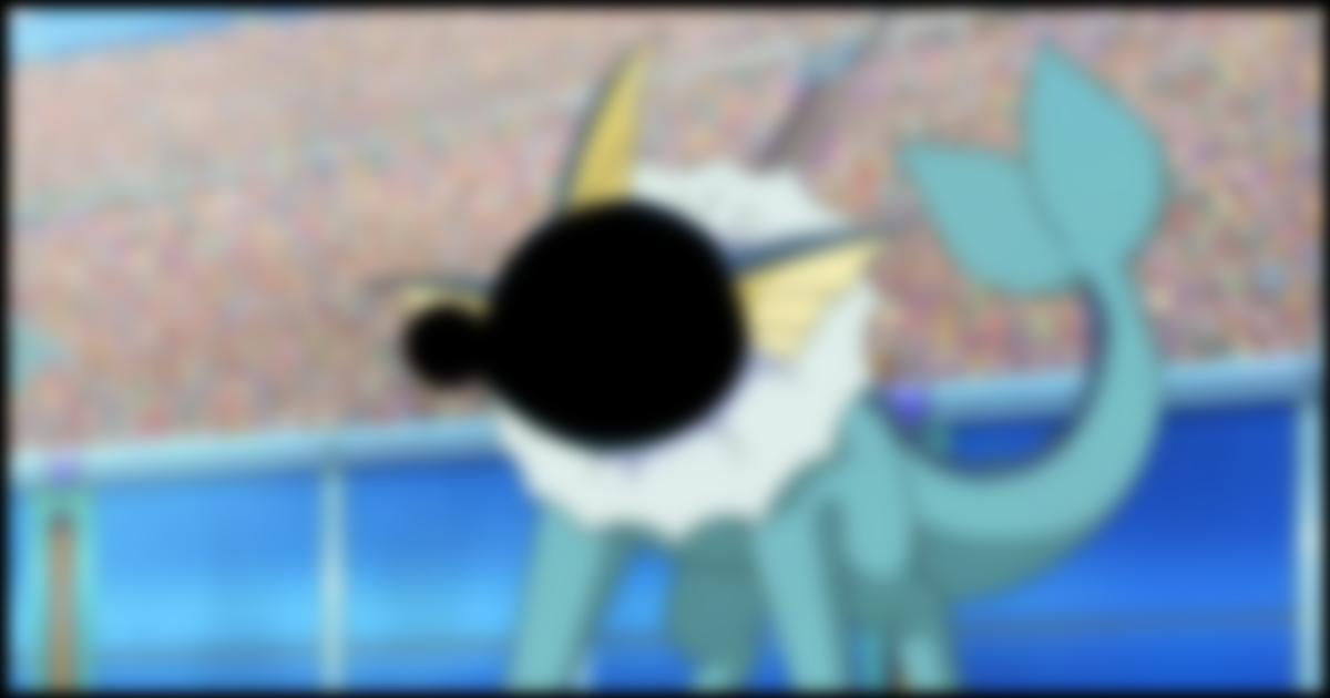
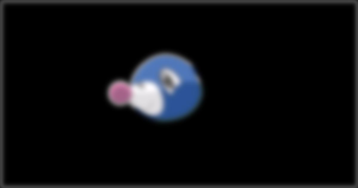
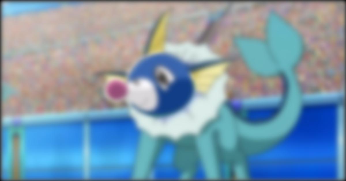
Vaporeon/Sylveon Combination (Failure)
Vaporeon

Sylveon
Vaporeon (Low Frequencies)
Sylveon (High Frequencies)
Combination (Sylporeon)
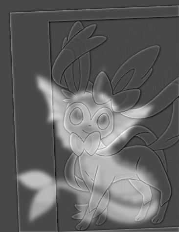
This combination likely failed due to the face structures of both pokémons being completely different, as well as their bodies not lining up at all, therefore making it hard to mesh the two together. As such, it is easy to discern both the low and high frequencies in the hybrid image at a close distance.
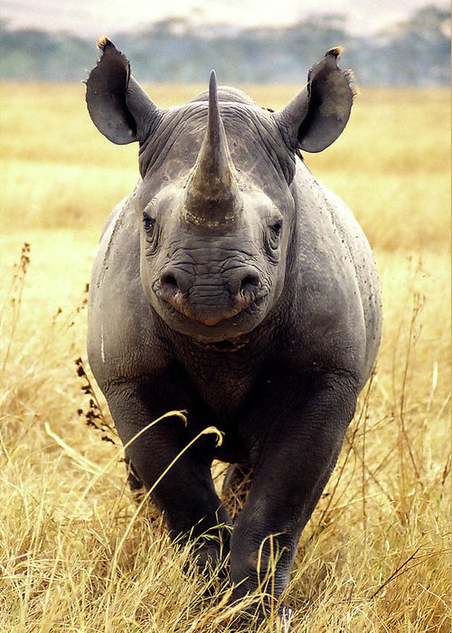
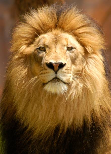
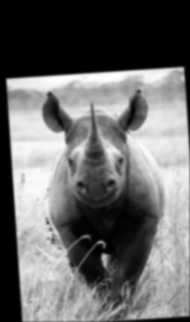
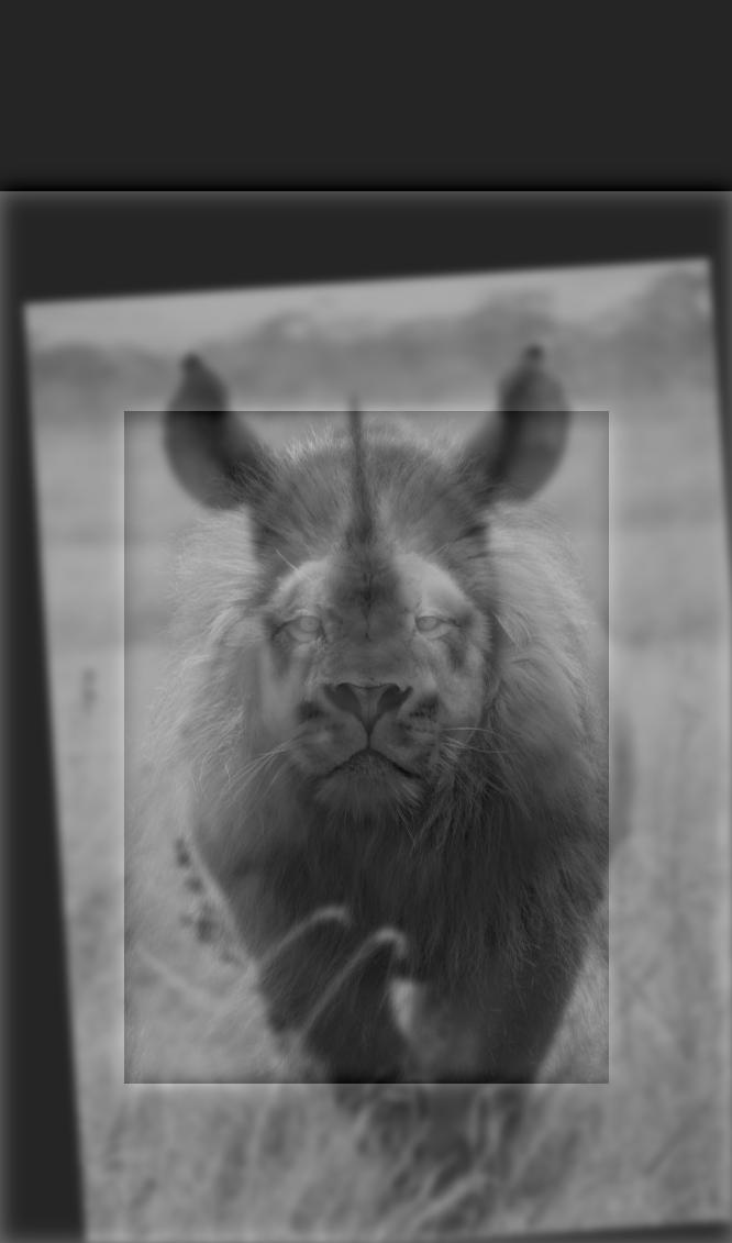
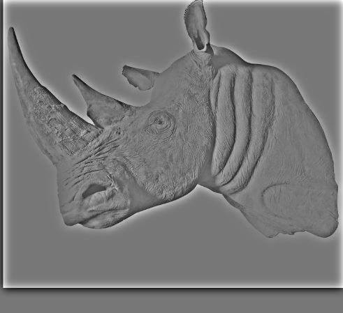
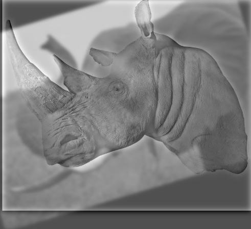
Rhino/Lion Combination (Best Custom Merge)
Rhino
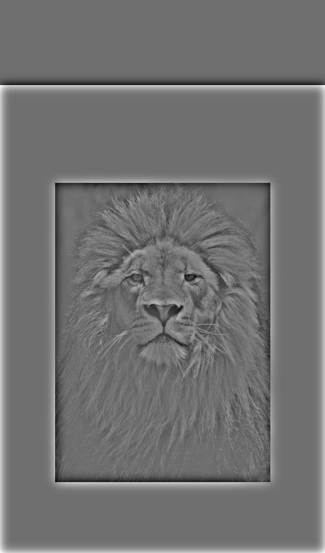
Lion
Rhino (Low Frequencies)
Lion (High Frequencies)
Combination (Lhino)
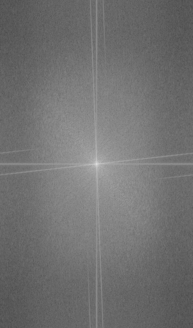
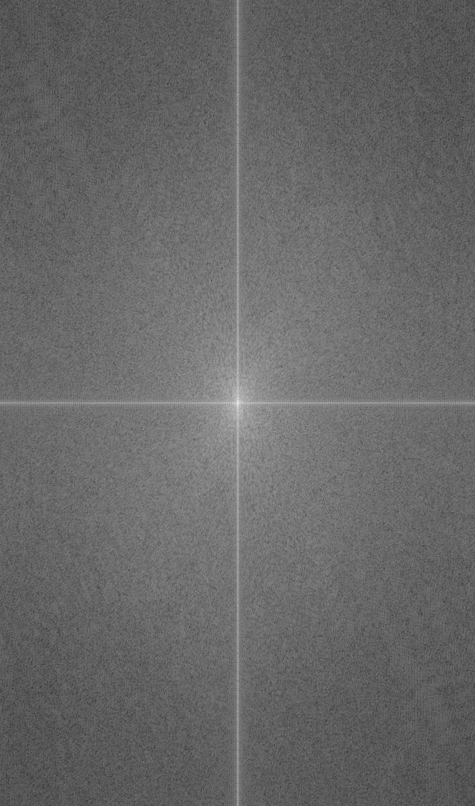
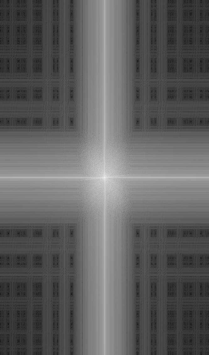
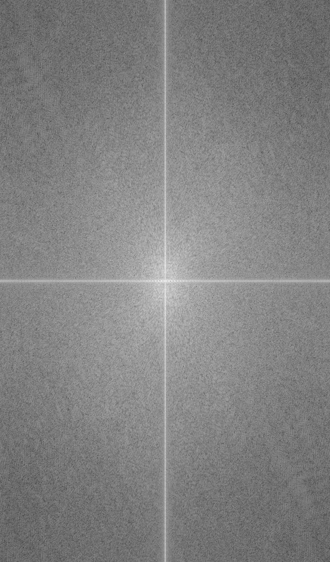
Listed below is the log magnitude of the Fourier transform for each of the individual images.
Rhino FFT
Lion FFT
Rhino (Low Freqs) FFT
Lion (High Freqs) FFT
Combination (Lhino) FFT
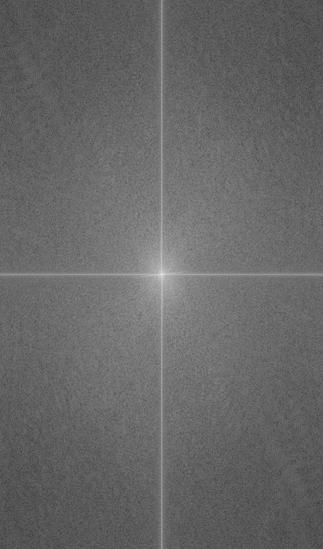
The success of this merge likely has to do with both the Rhino and Lion images sharing similar face structures, making it easy to overlay both images on top of each other. Additionally, as seen by the FFT images (where values closer to the origin represent lower frequency bases of the image), the blurred rhino does not contain many high frequency bases (the bases away from the origin are darkened and bases near the origin are amplified) whereas the high-frequency lion contains more brightness in bases away from the origin (those sections are brightened/amplified compared to the original image).
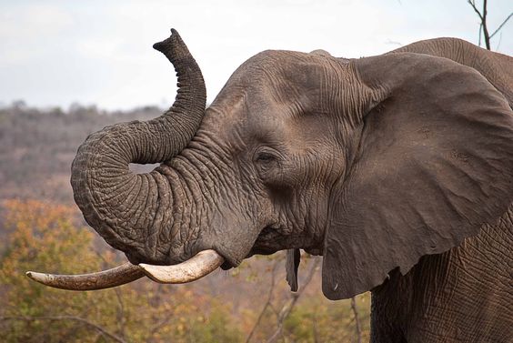
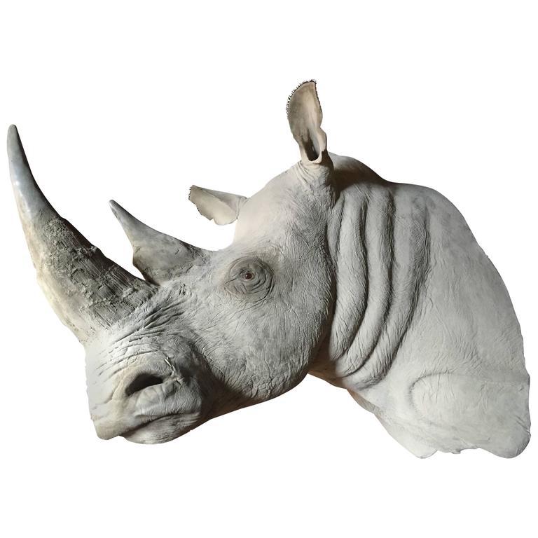
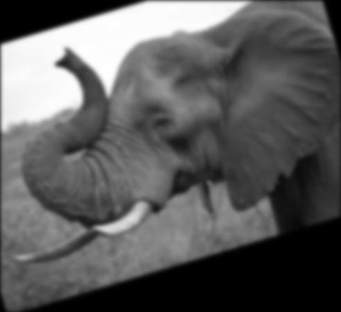
Elephant/Rhino Combination
Elephant
Rhino
Elephant (Low Frequencies)
Rhino (High Frequencies)
Combination (Elerhino)
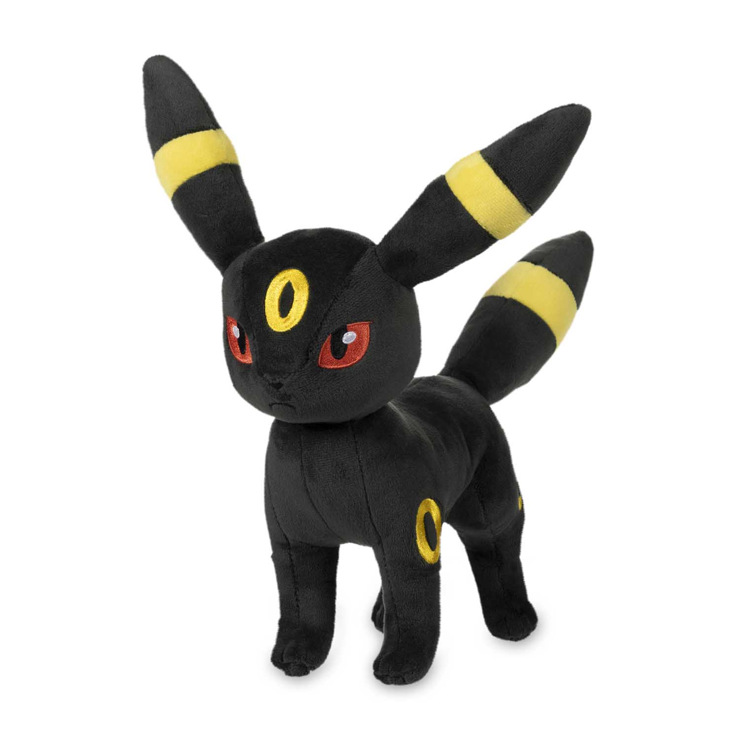
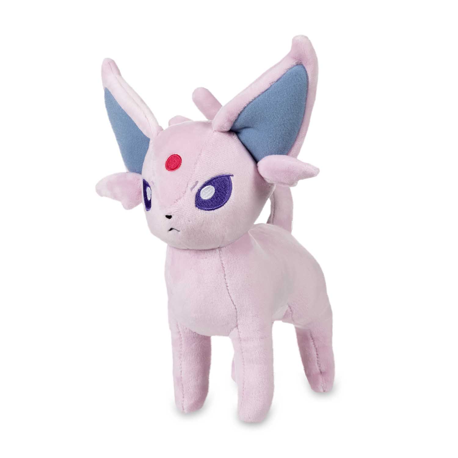
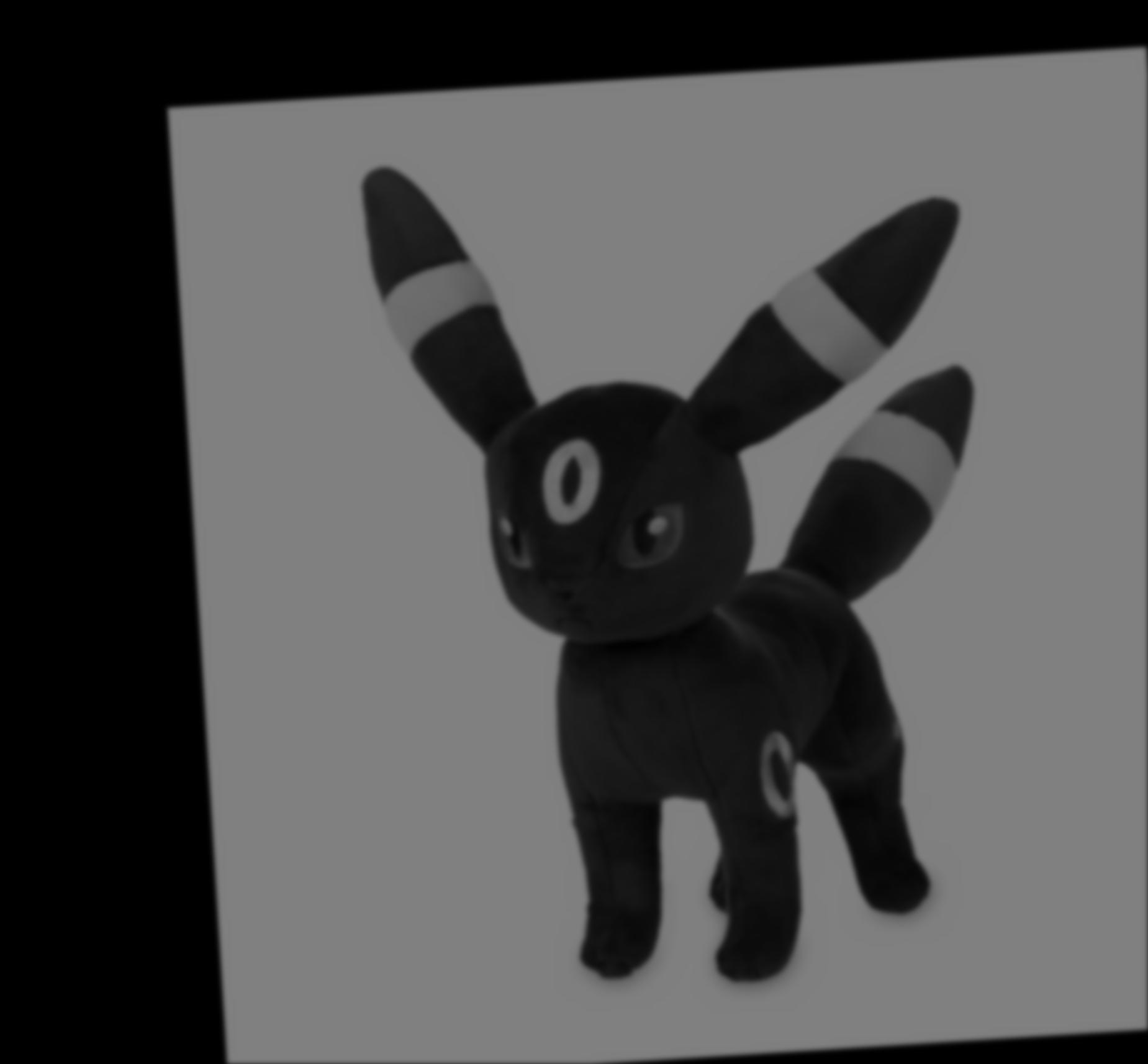
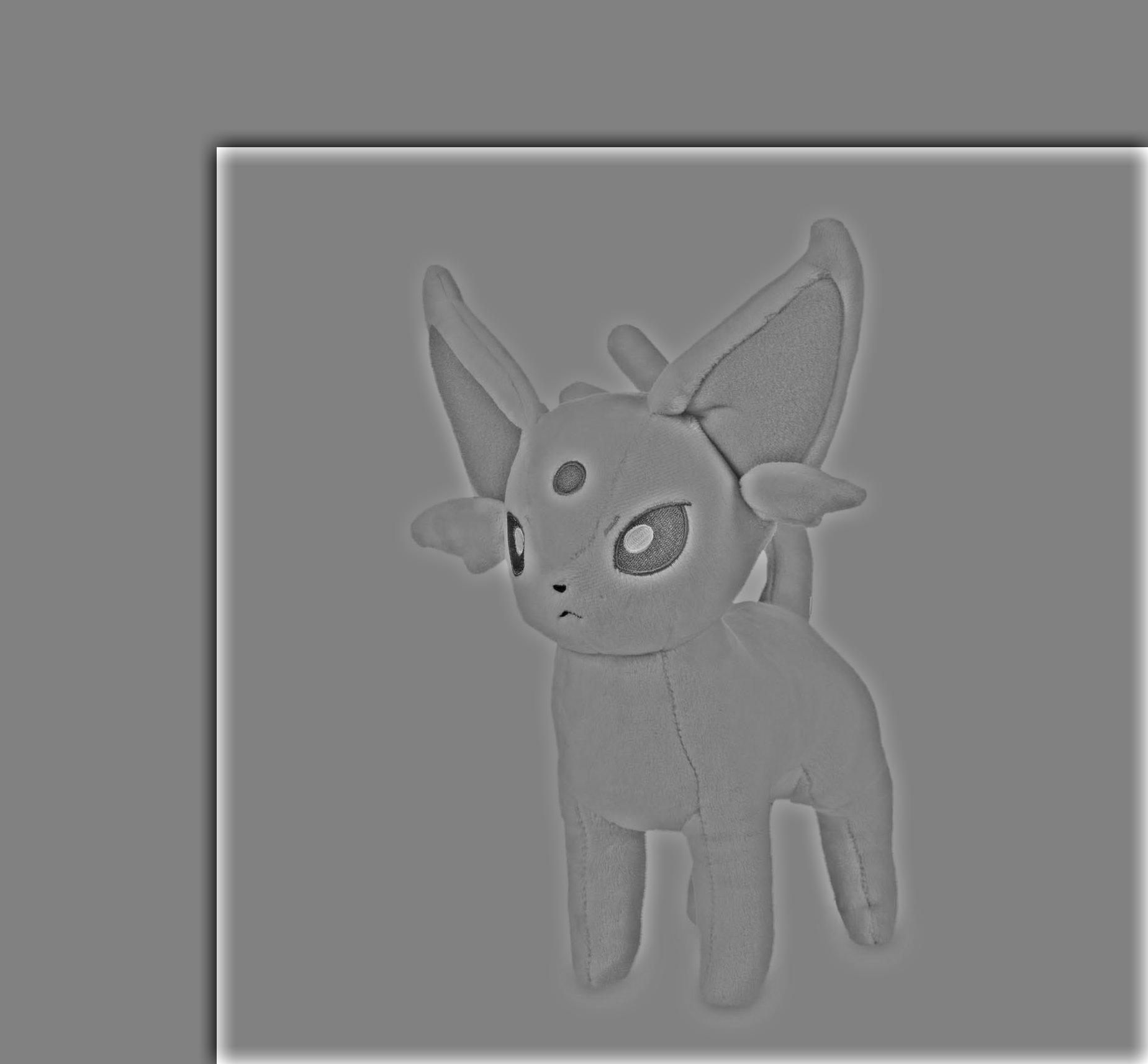
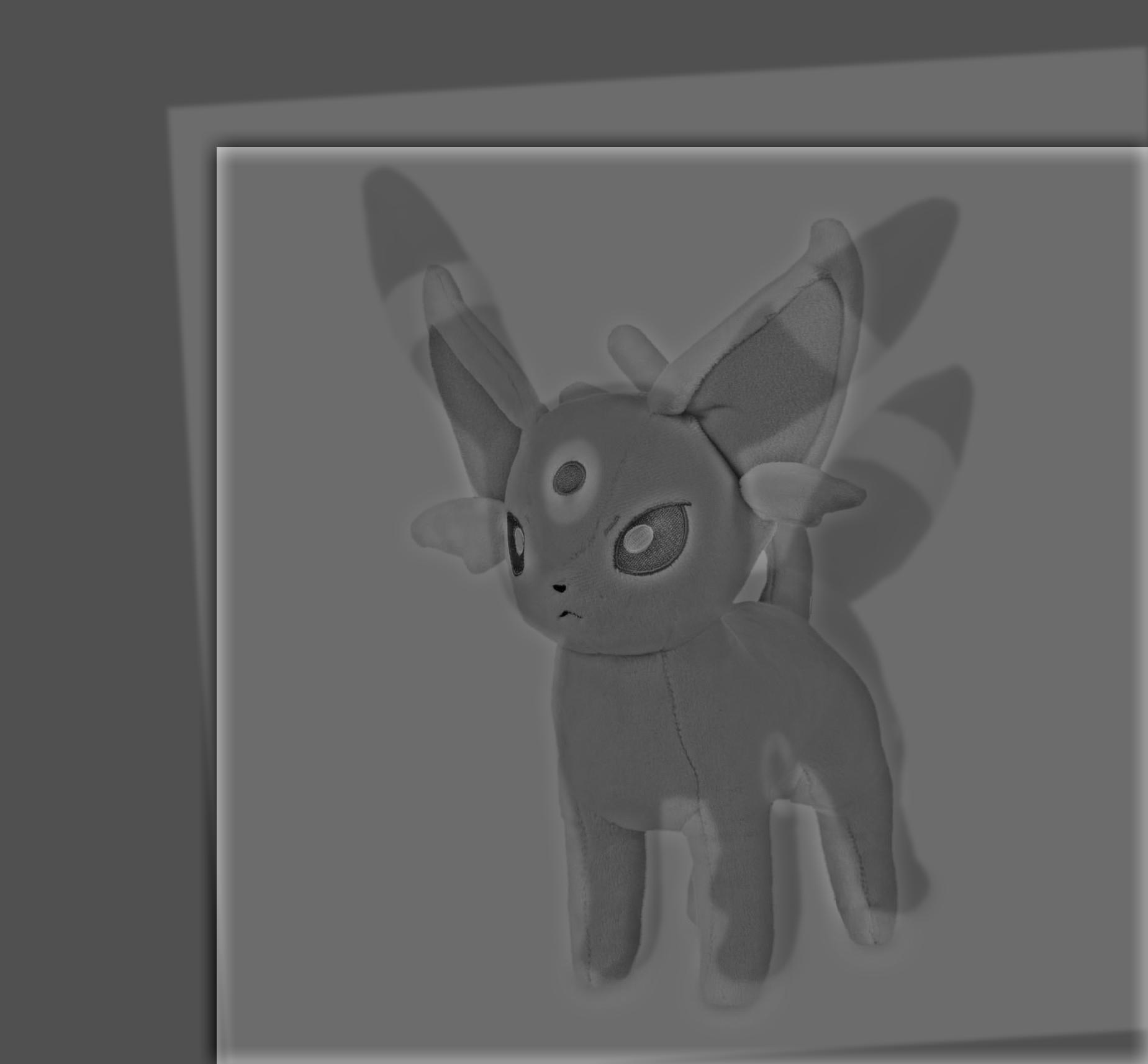
Umbreon/Espeon Plushie Combination
Umbreon
Espeon
Umbreon (Low Frequencies)
Espeon (High Frequencies)
Combination (Espreon)
Part 2.3: Gaussian and Laplacian Stacks
The task for this part was to implement a Gaussian and Laplacian stack. The Gaussian stack
is generated from an image being repeatedly blurred with a
Gaussian filter, where the sigma of the Gaussian filter doubles after each iteration. The
Laplacian stack is generated from the Gaussian stack, where the
ith image in the Laplacian stack is set equal to the result of gaus[i -
1] - gaus[i] (where gaus[i] is the ith
image in the Gaussian stack). Note that the last image in the Laplacian is the last image in
the Gaussian stack.
Each image in the Laplacian stack "encodes" the frequencies between two
corresponding images in the Gaussian stack.
Note that unlike a pyramid (where images are downsized at each iteration), the
Gaussian/Laplacian stacks do not downsize the image.
Additionally, the Gaussian/Laplacian stack must be processed individually on each color
channel of the image (R/G/B). The results below show the combined
result of merging the Gaussian/Laplacian stacks for each channel together into one image.
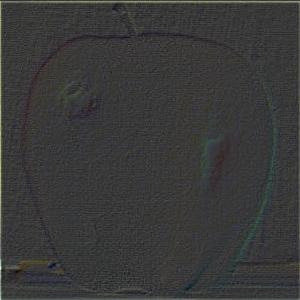
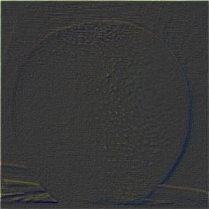
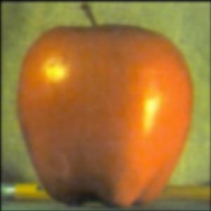
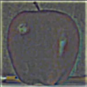
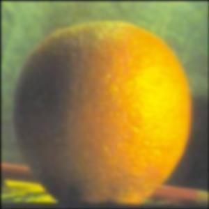
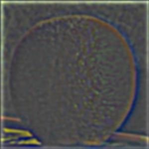
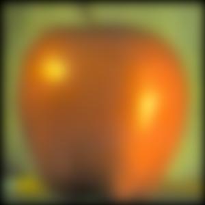
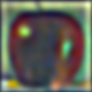
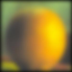
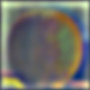
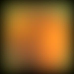
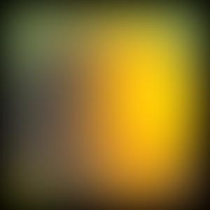
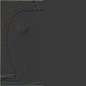
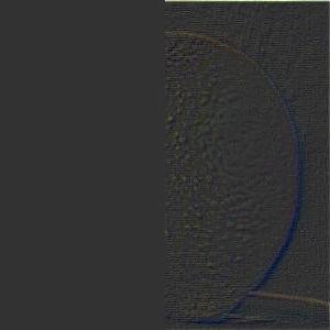
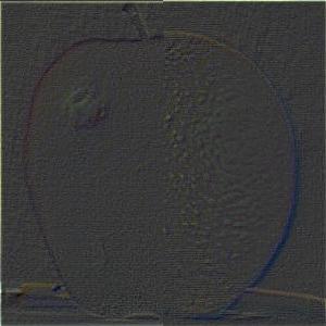
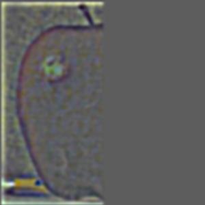
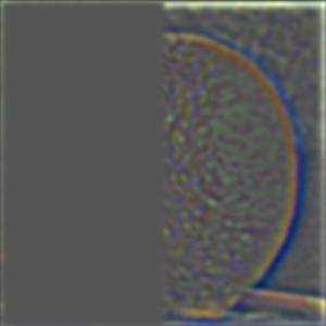
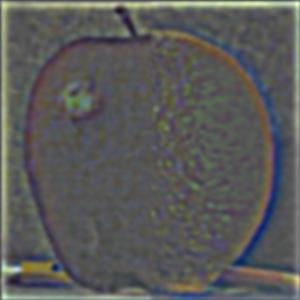
7-Layer Apple/Orange Gaussian/Laplacian Stack (Layers 0, 2, 4, 6 Shown)
Apple
(Gaussian)

Apple
(Laplacian)
Orange
(Gaussian)
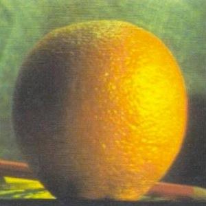
Orange
(Laplacian)


Part 2.4: Multiresolution Blending (A.K.A. the Oraple!)
Taking the results from part 2.3 (building the Gaussian/Laplacian stacks), we can combine
the Laplacian stacks of both images to blend
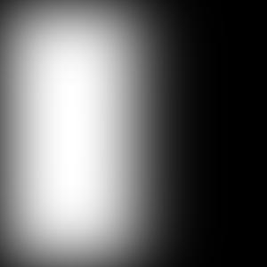
them together. To do this, we first initialize a mask with only 0 and 1 values that
indicates which pixels from either image to include.
After, we generate the Gaussian stack for the mask and Laplacaian stacks for each image we
are blending.
To build our image, we first initialize a matrix imgout with all 0's that
matches the dimensions of the images we are merging. Let mask
be the array that contains the Gaussian stack for the mask and La and
Lb represent arrays for the Laplacian
stacks of image A and image B.
For every image number i in each stack: imgout += mask[i] *
La[i] + (1 - mask[i])
* Lb[i]
In essense, we are adding all the Laplacian layers together but filtering each image by the
pixels inside the mask. Using a Gaussian stack for the mask
generates a "blur" effect at the seam for both different images, creating a perfect blend!
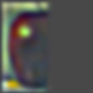
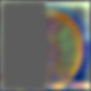
7-Layer Gaussian/Laplacian Stack with Mask (Layers 0, 2, 4, 6 Shown)
Mask
(Gaussian)

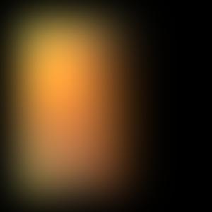
Apple * Mask
(Laplacian)
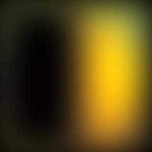
Orange * (1 - Mask)
(Laplacian)
Together
(Laplacian)


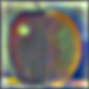
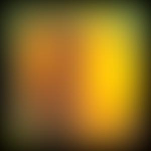
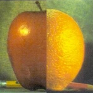
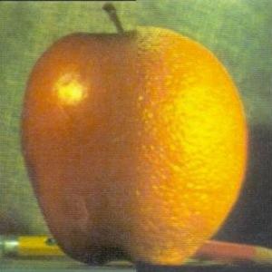
Final Result (Oraple)
Unblurred
Blurred
Listed below are some other images that were blended together along with the corresponding mask.
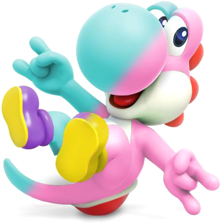
Blue/Pink Yoshi
Blue Yoshi
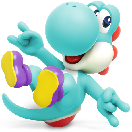
Pink Yoshi
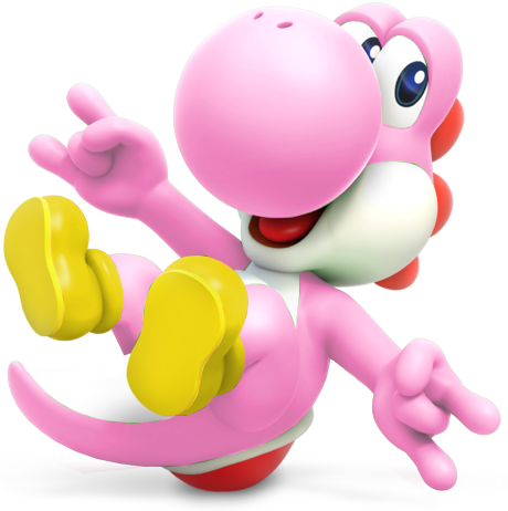
Mask
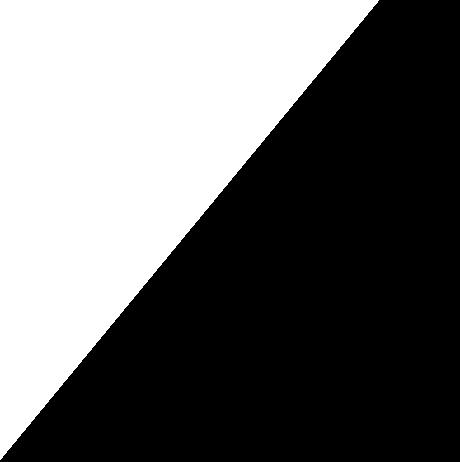
Result
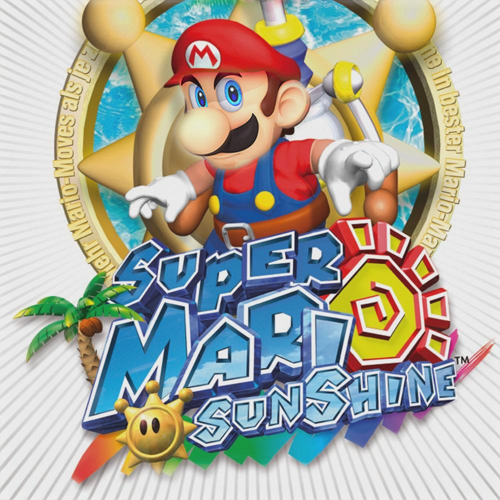
Mario/Luigi Sunshine
Mario
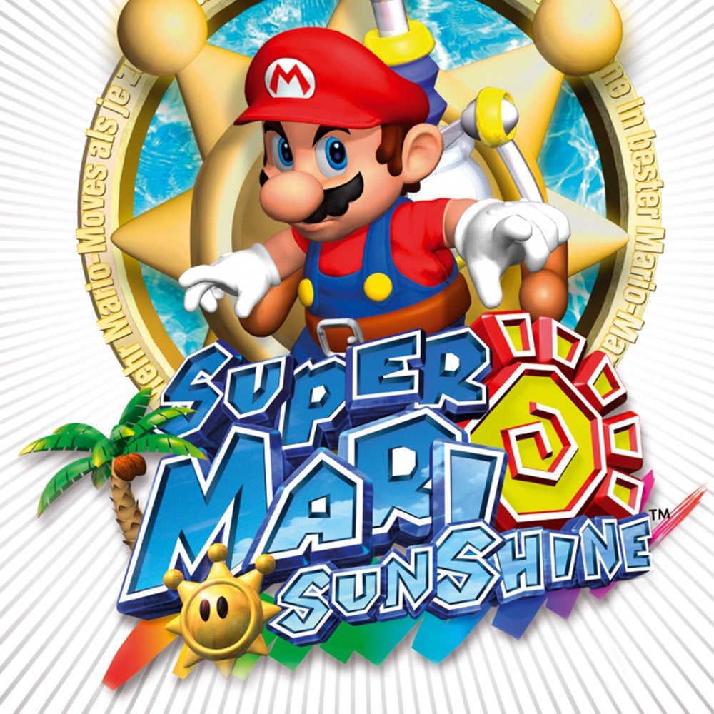
Luigi
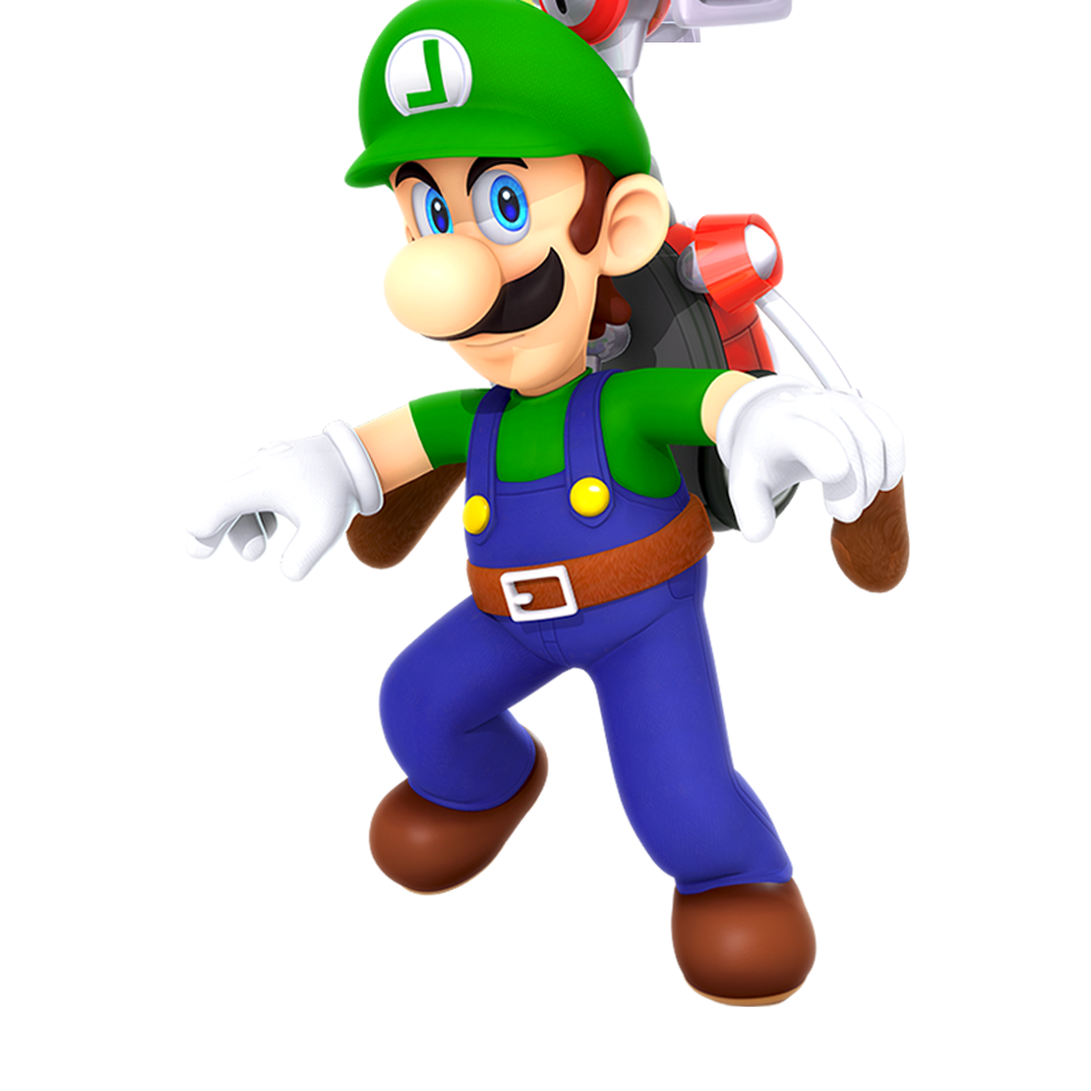
Mask
Result
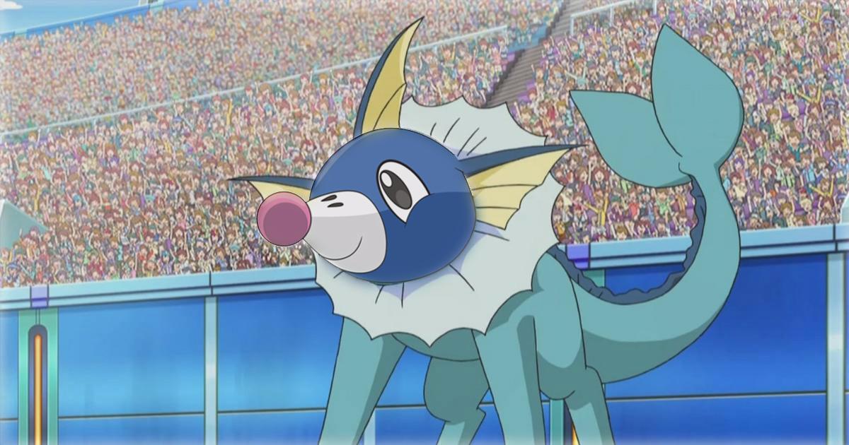
Vaporeon/Popplio Merge (Vapplio)
Vaporeon
Popplio

Mask

Result
5-Layer Gaussian/Laplacian Stack for "Vapplio"
Mask
(Gaussian)
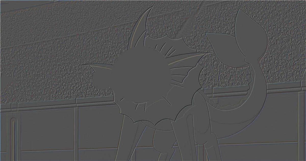
Vaporeon * Mask
(Laplacian)
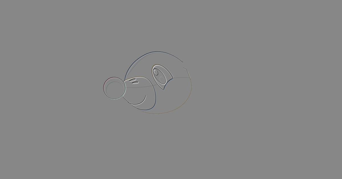
Popplio * (1 - Mask)
(Laplacian)
Together
(Laplacian)


Conclusion
Overall, I had a really fun time working on this project, and I was shocked by how something as simple as a Gaussian blur filter could be utilized in so many different ways, including the unsharp mask filter (which sounded counterintuitive at first). I especially enjoyed being able to create my own hybrid images and experimenting with "hyperparameters" (i.e. Gaussian sigma, different image alignments, etc.) to find the combination that yielded the best results. Additionally, it was satisfying to look at the separate layers in the Gaussian/Laplacian stacks and seeing how they could all be combined into one blended image.