Project 5: Facial Keypoint Detection with Neural Networks
Project Overview
In previous projects, we needed to manually detect keypoints in order to perform most of our transformations.
Therefore, the goal of this project is to train a series of neural networks that can automatically detect
facial keypoints for us!
Project Link
Part 1: Nose Tip Detection
To ease ourselves into the project, let's attempt to detect the nose tip among a collection of
images from the IMM Face Database.
The images of the first 32 individuals were used as the training set and the remaining 8 as the validation set, with
each individual having a series of 6 images. We process these inputs by coverting the image into grayscale, then downsizing the image to 80 x 60.
Below is a set of training images and their corresponding nose tip labels.
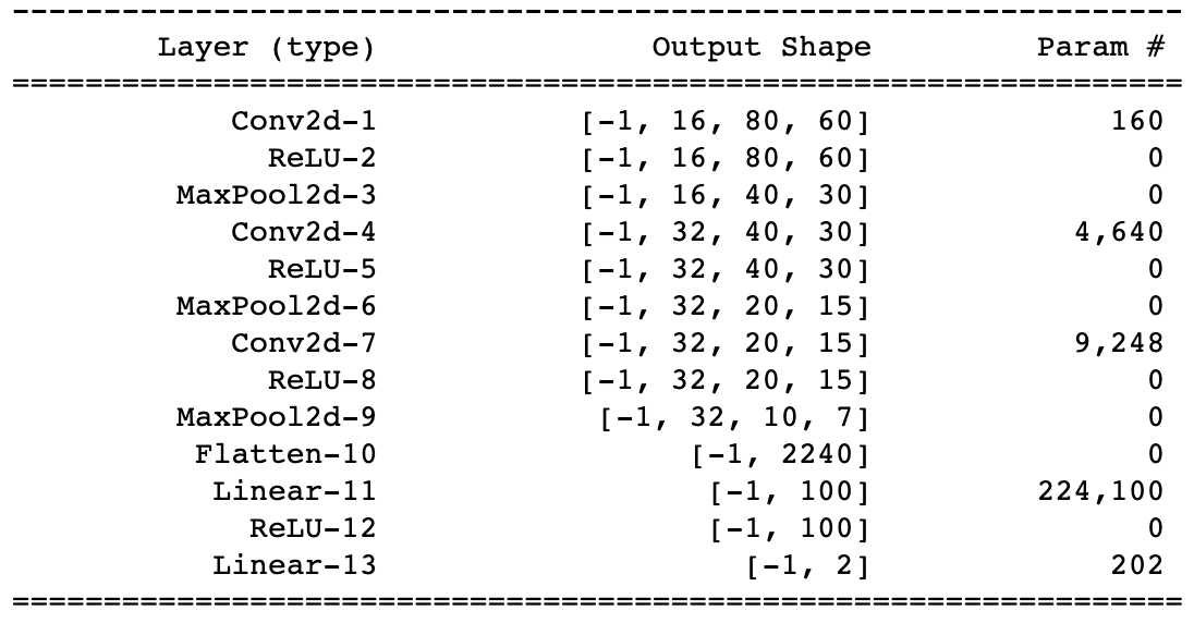
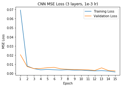
A summary of the CNN used for this part is shown to the left, with the output being a 2-item tensor that contains xpred and ypred values of the nose tip in ratio form (i.e. to recover the original coordinates (x, y), calculate x = xpred * width_of_image and y = ypred * height_of_image). The network was trained using the Adam optimizer with a learning rate of 1e-3 and mean squared error loss (MSE). The training/validation MSE loss per epoch is shown to the right.
Model Summary
Training/Validation MSE Loss
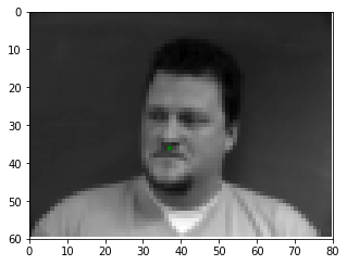
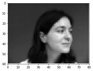
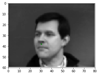
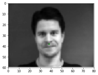
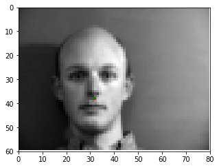
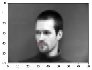
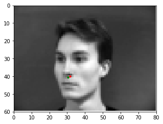
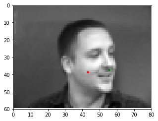
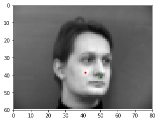
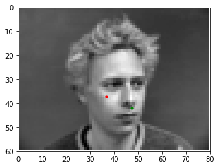
Here are some examples of the network performing on the validation set with the red point as the model's prediction and the green point as the ground truth. Note that the network seems to perform well on faces that are either facing forwards or turned to the left, but perform poorly on faces that are turned to the right. This may be caused by the model showing biased towards predicting keypoints on the left portion of the image.
Good Match 1
Good Match 2
Good Match 3
Bad Match 1
Bad Match 2
Bad Match 3
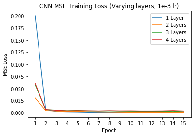
Additionally, we can try varying different hyperparameters of the network to see if these changes have any impacts on the network performance. For this exercise, I decided to vary the number of convolutional layers (we used 3 Conv layers in the default model) and the learning rate for the Adam optimizer (we used 1e-3 in the default model).
Varied Layers, Training Loss
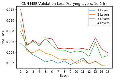
Varied Layers, Validation Loss
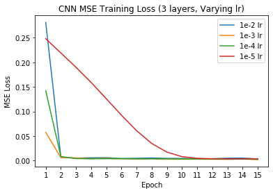
Varied Learning Rate, Training Loss
Varied Learning Rate, Validation Loss
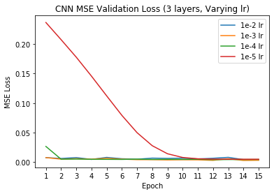
When varying the number of layers, it appears that having less convolutional layers performs much better on the validation set in terms of MSE loss - this may be due to the prediction task not being very difficult (only predicting two coordinates x and y); thus a simple model suffices well. Additionally, although varying the learning rate doesn't change the performance of the model (all models eventually converge around the same training and validation MSEs), it does impact how long it takes for the model to reach convergence, with the lower learning rates (1e-4 and 1e-5) taking much longer to converge.
Part 2: Full Facial Keypoints Detection
Expanding from the previous part, we will now train a model to detect all 58 keypoints on each individual
given the same IMM Face Database.
Given that this is a small dataset, it may be beneficial to apply data augmentation to prevent the model from overfitting
on the training set. We can achieve this by modifying the brightness of the image, rotating the image (from -15 to 15 degrees),
and shifting the image (10-15 pixels along both directional axes).
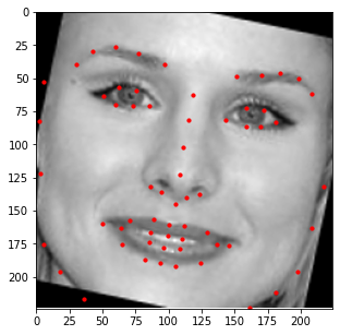
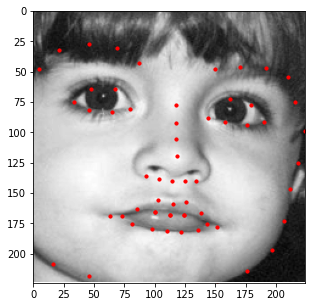
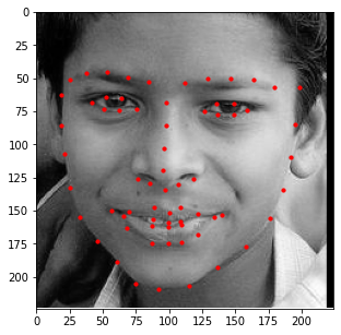
Below is a set of the augmented training images and their ground truth labels.
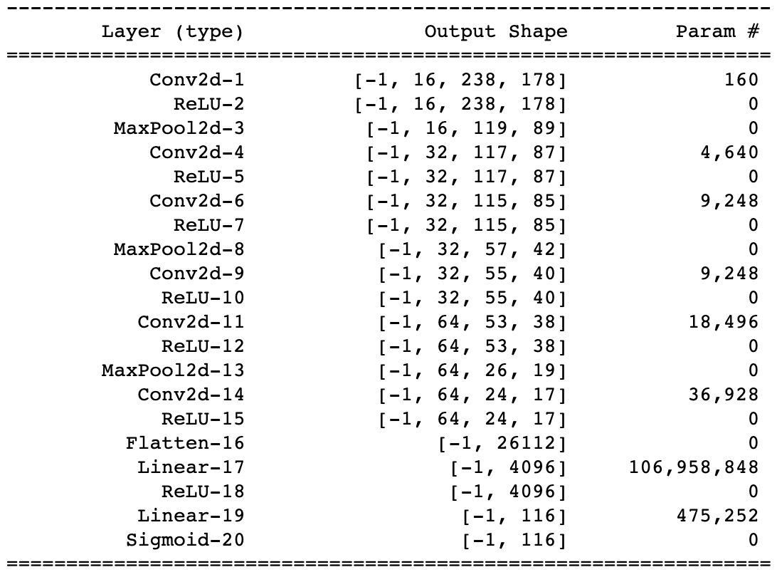
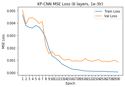
A summary of the CNN used for this part is shown to the left, with the output being a 116-item tensor that contains 58 sets of (x, y) coordinate pairs of the entire face in ratio form (similar to part 1). The network was trained using the Adam optimizer with a learning rate of 1e-3 and mean squared error loss (MSE). The training/validation MSE loss per epoch is shown to the right.
Model Summary
Training/Validation MSE Loss
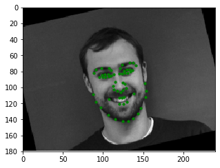
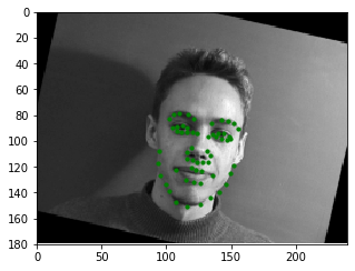
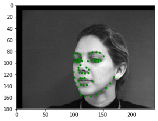
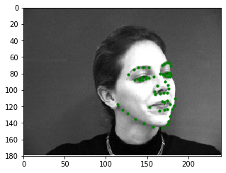
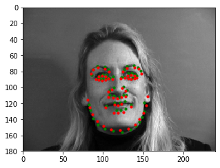
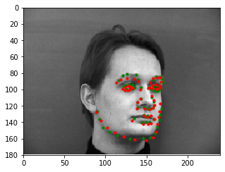
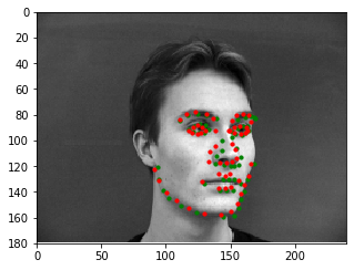
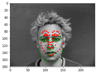
Here are some examples of the network performing on the validation set with the red points as the model's prediction and the green points as the ground truth. Note that the network seems to perform well on faces that are either facing forwards or turned to the right, but perform poorly on faces that are turned to the left. Additionally, there are a couple of outlier images that aren't classified well when the individual's eyes are wide open - this may cause the model to interpret the person's eyebrows as the face's eyes.
Good Match 1
Good Match 2
Good Match 3
Bad Match 1
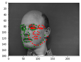
Bad Match 2
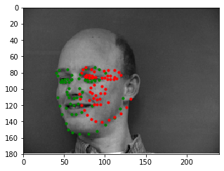
Bad Match 3
Additionally, here are some visualizations of the 3x3 filters at different convolutional layers. It's difficult to tell what each individual filter is trying to detect within the image, but they all work together to detect specific characteristics of each image that allows one to detect keypoints within it. (Note, some of the images are very large)
Layer 1 (1 x 16)

Layer 3 (16 x 16)
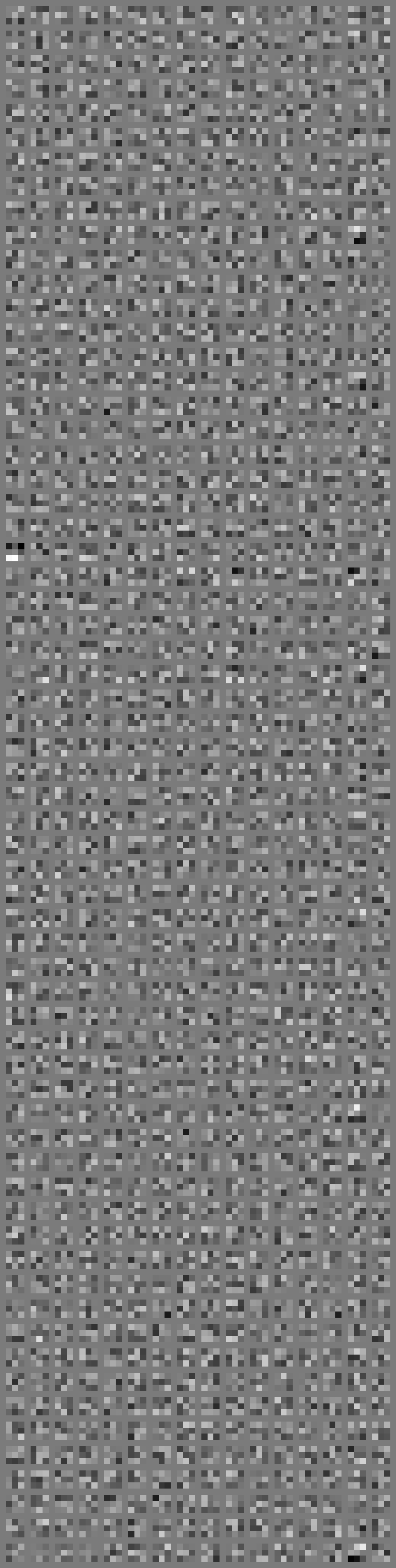
Layer 5 (32 x 32)

Part 3: Train With Larger Dataset
Now let's tackle a larget dataset! For this part, we are given the ibug face in the wild
dataset and are tasked with training a model to predict 68 different keypoints on each
one of these images. We were given 6666 images to train the model with, and I split 80%
of the data into a training set and the remaining 20% into a validation set.
To process each image, I used the provided bounding box to crop the image to focus on the individual's
face, then resized that cropped image to 224x224. The image is then converted to grayscale. Additionally, similar to part 2,
the images in the training set were also transformed with random rotation, scaling, and brightness changes.
The visualization of some training samples are shown below. Note that some of the keypoints fall outside of the
provided bounding box, but this is not an issue for the CNN model since it can predict negative coordinate ratios.
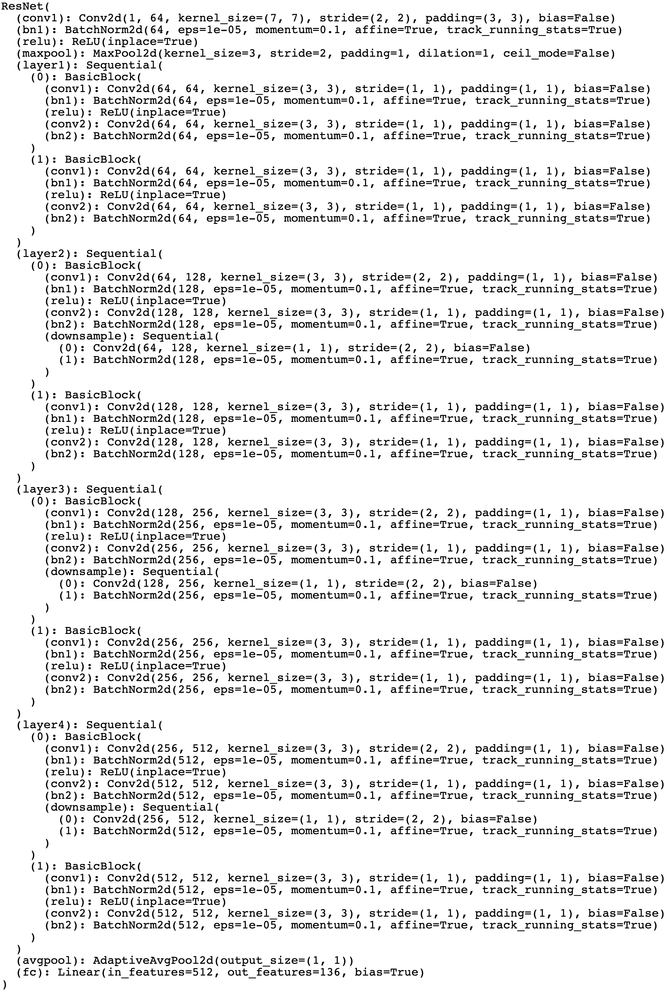
For this part, I decided to use a state-of-the-art model called
ResNet-18
to learn the keypoints of each image. Note that small parts of this model were tweaked to conform with
the desired input and output sizes (1 input channel for input due to having a grayscale image, 68 * 2 = 136 output
channels given that we're trying to detect 68 keypoints).
A summary of the CNN used for this part is shown to the left, with the output being a 136-item tensor
that contains 68 sets of (x, y) coordinate pairs of the entire face in ratio form (similar to parts 1/2).
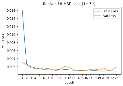
The network was trained using the Adam optimizer with a learning rate of 1e-3 and mean squared error loss (MSE). Note
that the model was trained for 23 epochs - it was intended to train the model for 30 epochs but I was forced to stop
training due to running out of GPU credits on Google Colab.
The training/validation MSE loss per epoch is shown to the right.
Model Summary
Training/Validation MSE Loss
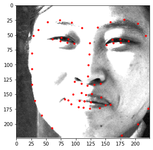
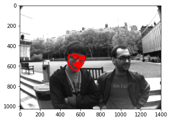
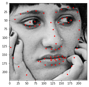
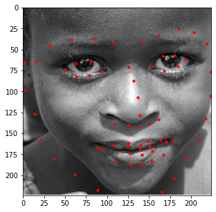
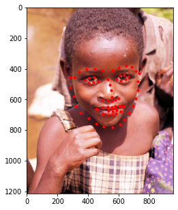
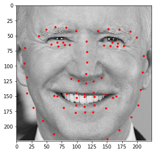
In order to test the performance of the model, 1008 images without labels were provided to serve as a test set.
Below are some results of the model being executed on the test set with both the bounding box (left) and
expanded image (right). Overall the performance isn't that bad!
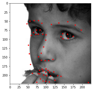
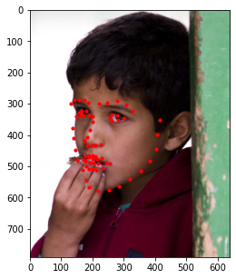
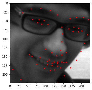
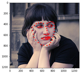
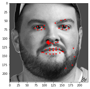
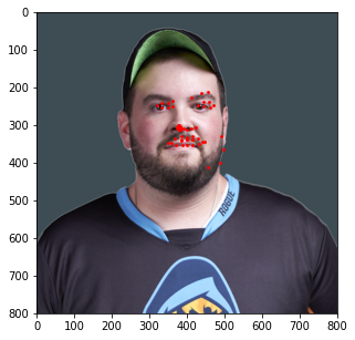
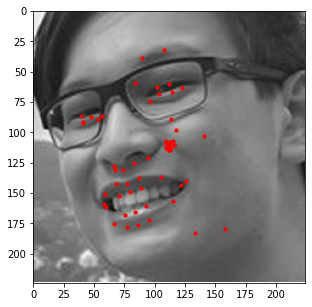
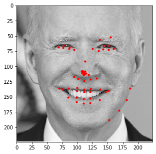
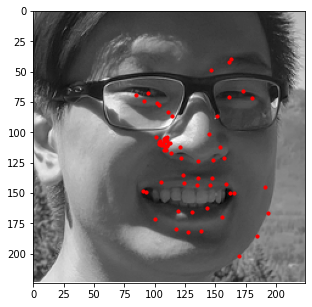
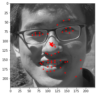
Additionally, I decided to run this model on a few images of my own. Those results are shown below.
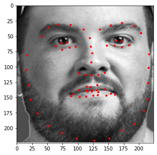

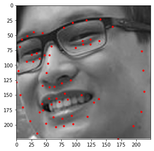
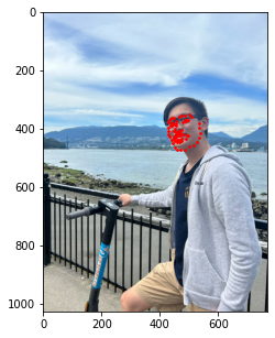

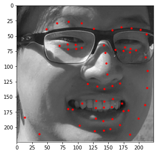
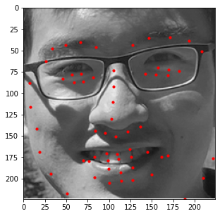
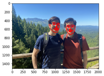
In general, it seems like the model does a great job at detecting the general shape of each person's face and the general placement of each individual's features (i.e. mouth, nose, etc.); however, the exact details of these features seem slightly off (especially when detecting eyes). This could be due to other artifacts being present (like eyebags or glasses) which makes this specific kind of detection difficult for the model. As such, a larget dataset that captures these details would be beneficial should we decide to train the model again.
Part 4: Pixelwise Classification
Now let's try utilizing a different model to achieve the same task as part 3. Instead of outputting
136 (x, y) ratio vaues for each image, let's instead train a model to output a 224 x 224 heatmap for each keypoint in
the image (68 heatmaps total). Each heatmap will encode probabilities indicating how likely it is for
the keypoint to be located at a specific coordinate. As such, we can take a weighted average over
each generated heatmap to recover the (x, y) ratio values generated by the model.
To generate a ground truth heatmap for one keypoint, we place a Gaussian kernel with a kernel size of 19 and a sigma of 3
centered around the keypoint and zero out the rest of the canvas - as such, the only non-zero values in the ground truth heatmap come from the Gaussian
kernel. We repeat this process for all 68 keypoints to generate 68 "ground truth" heatmaps. An example of an aggregated
heatmap overlayed a few of the augmented training images are displayed below.
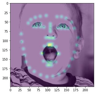
Note that this method of model training only works if all keypoints are within the bounding box. As such, I expanded every bounding box by a factor of 1.25 and threw out all training data that did not have its keypoints within the expanded bounding box.
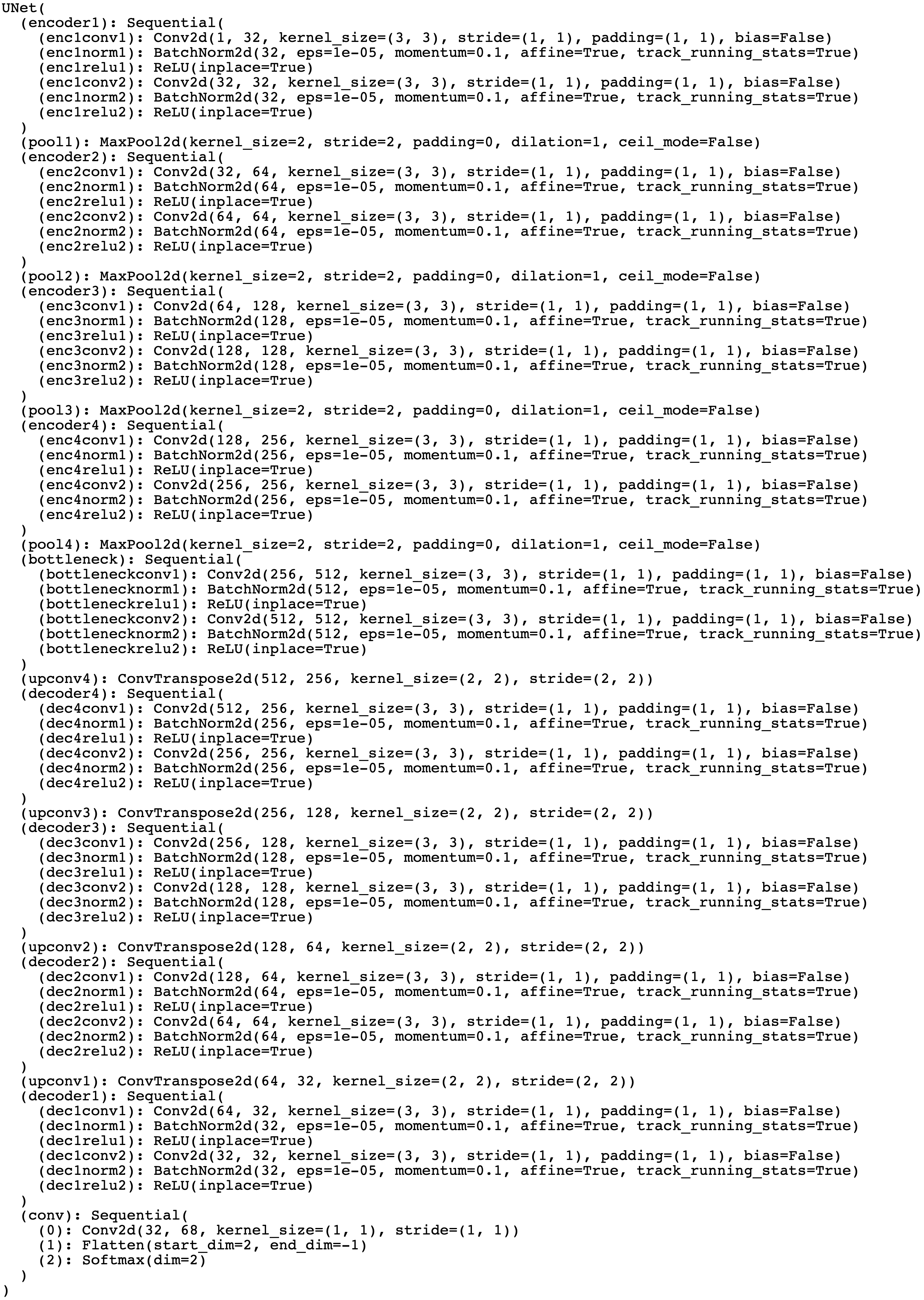
The model utilized for this part is a state-of-the-art UNet
CNN. Similar to the previous part, I modified the model to take in one input channel (grayscale image) and output 68 flattened
heatmaps (output tensor of 68 x (224 * 224) = 68 x 50716). Additionally, I modified the model to take a softmax over each heatmap such that the outputted values in the
model sum to 1 to represent probabilities of each keypoint. The network was trained using the Adam optimizer and mean squared error loss (MSE) over
the converted (x, y) ratios generated by taking the weighted average over each heatmap.
Initially, the model was training using a learning rate of 1e-3; however, as the model continued to train, I kept increasing the learning rate
due to the model taking a very long time to converge. The following list indicates what learning rate was used for specific epochs during the training process:
- Epochs 1 - 18: 1e-3
- Epochs 19 - 27: 3e-3
- Epochs 28 - 34: 4e-3
- Epochs 35 - 49: 6e-3
- Epochs 35 - 88: 8e-3
Model Summary
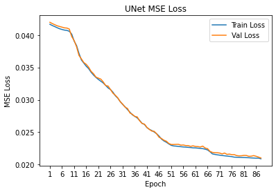
Training/Validation MSE Loss
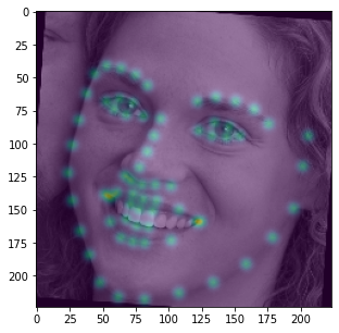
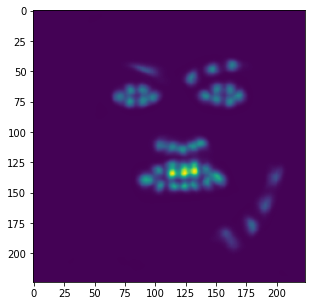
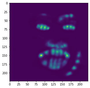
Similar to the previous part, I also evaluated the performance of this model on the provided test
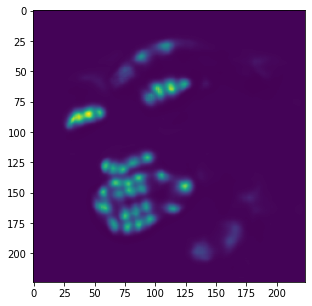
images in the ibug dataset. Some examples of these results are shown below with an aggregated
heatmap and its calculated keypoints.
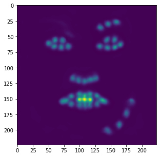
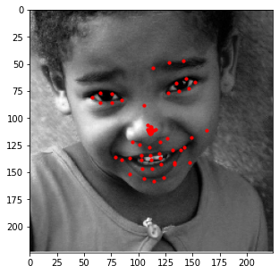
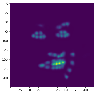
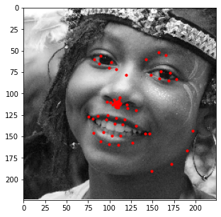
Unfortunately, these results aren't as great as the previous part. Although this model is very good at identifying facial features (eyes, nose, teeth, right eyebrow), it completely fails to detect the outer face of each individual, most of these keypoints being clumped together in the middle. In retrospect, using a higher learning rate or different form of error (i.e cross entropy instead of MSE) could have maybe prevented this from happening, as most of the outer keypoints weren't able to converge to the right values despite training the model for almost 100 epochs.
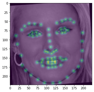
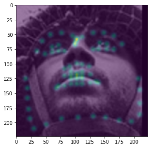
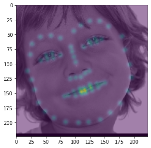
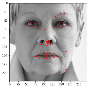
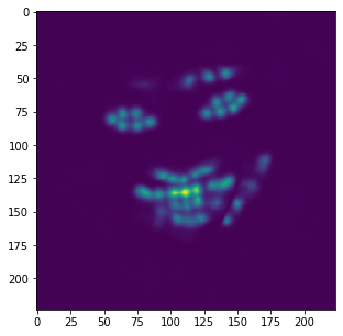
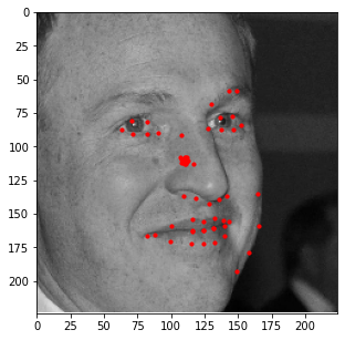
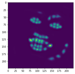
Similar to the last part, here is the model's performance on some of my own images:

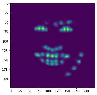
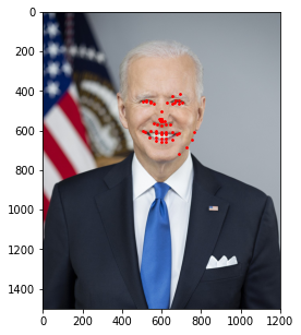
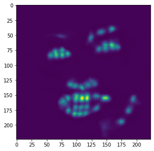

Similar to the previous example, the correct features are strikingly accurate; however, it is obvious that there are a few features that model has failed to learn.
Part 5: Kaggle
I submitted my test results from part 3 to this semester's Kaggle competition, as my ResNet results were much better than the UNet. My username is brywong and the MSE I achieved was 11.59006, currently among the top half of the class.