CS194 Project 5:

[Auto]Stitching Photo Mosacis

Ahmed Malik || Spring 2020

Part A: Image Warping and Mosaicing

Overview

In this first part of project 5, we demonstrate two applications of perspective warping. First, we show image rectification by taking a picture of a planar surface, off-axis, and warping it such that the plane is frontal-parallel. Second, we blend two images taken from different view directions with some overlapping fields of view, effectively creating a mosaic or panorama of a larger field of view. The pixel positions of the warped images are determined by using a homography matrix.

Recovering Homographies

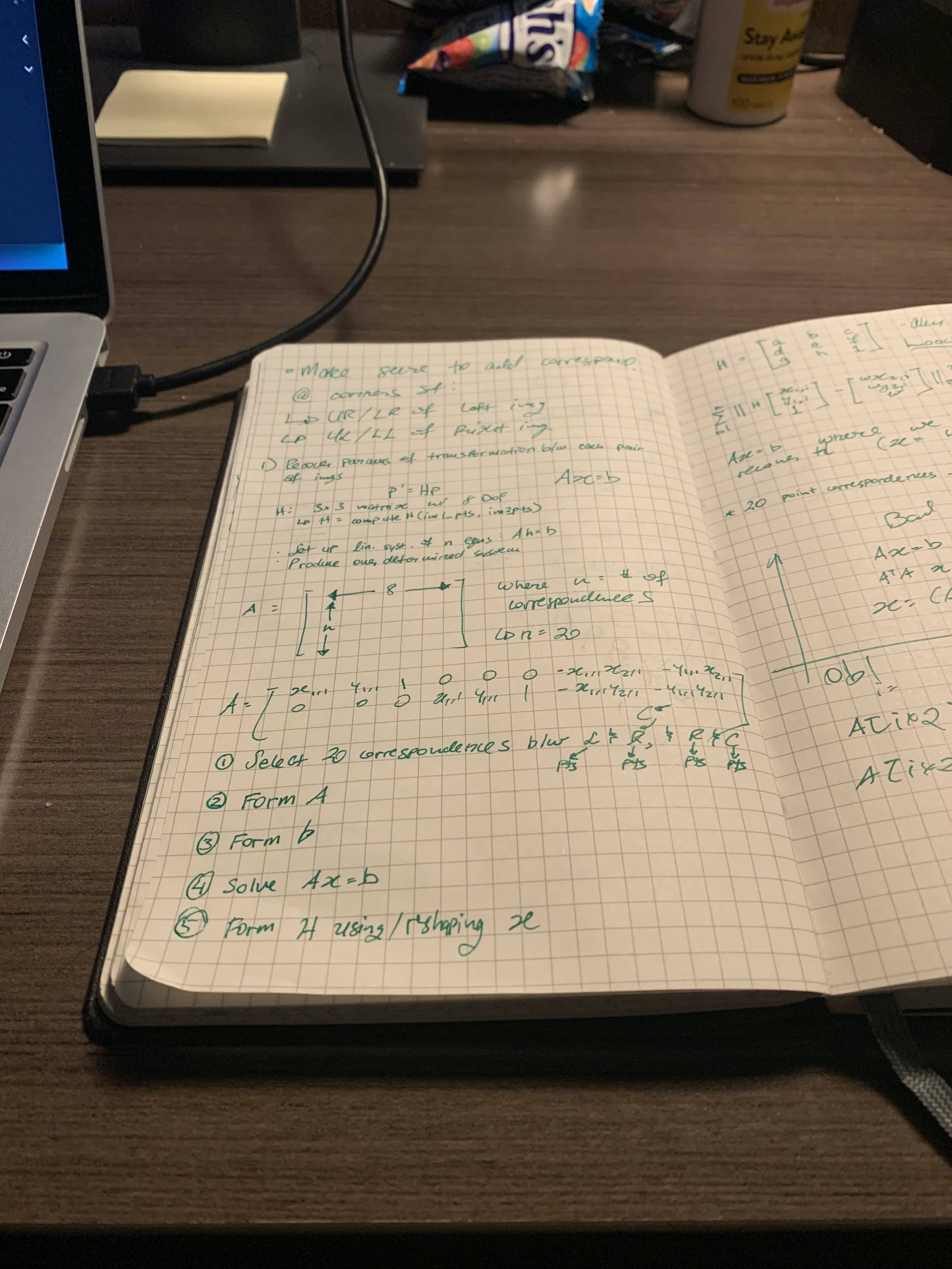
For the perspective warp, the first image is warped to the perspective of the second image. This is a homography where the new pixel locations p' are determined by a transformation of the original pixel locations p using a homography matrix: p'=Hp. The homography matrix H is a 3x3 matrix where the last element is always 1, meaning the matrix has 8 degrees of freedom (DoF). H is computed by taking points of correspondences between the original image and the perspective of the image it is being warped to, such that n linear equations are set up where n is the number of points of correspondence. Given that H has 8 DoF, only 4 points of correspondence are needed; however, more points of correspondence help reduce error in the homographies recovered. This can be formulated as Ah=b where A is the matrix composed of points of correspondences, h is an 8x1 vector for the 8 DoFs of H, and b is the vector composed of all the correspondences in the second image. This is shown below:

H = [\begin{matrix} a & b & c \\ d & e & f \\ g & h & 1 \end{matrix}]

[\begin{matrix} x_{1, 1} & y_{1, 1} & 1 & 0 & 0 & 0 & - x_{1, 1} x_{2, 1} & - y_{1, 1} x_{2, 1} \\ 0 & 0 & 0 & x_{1, 1} & y_{1, 1} & 1 & - x_{1, 1} y_{2, 1} & - y_{1, 1} y_{2, 1} \\ ⋮ \\ x_{1, n} & y_{1, n} & 1 & 0 & 0 & 0 & - x_{1, n} x_{2, n} & - y_{1, n} x_{2, n} \\ 0 & 0 & 0 & x_{1, n} & y_{1, n} & 1 & - x_{1, n} y_{2, n} & - y_{1, n} y_{2, n} \end{matrix}] [\begin{matrix} a \\ b \\ c \\ d \\ e \\ f \\ g \\ h \end{matrix}] = [\begin{matrix} x_{2, 1} \\ y_{2, 1} \\ ⋮ \\ x_{2, n} \\ y_{2, n} \end{matrix}] .

Thus, using least squares, we can solve for h and reshape it to form H. For part A of this project, the points of correspondence were all selected manually using ginput().

Image Rectification

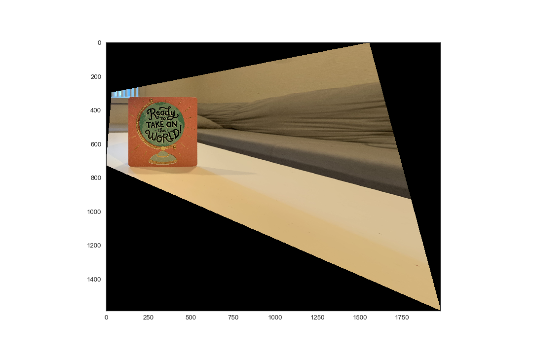
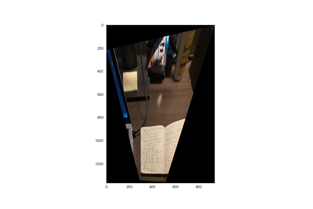
In this section, we warp an image of a planar surface such that it is frontal-parallel. The perspective transformation is performed using inverse image warping, and thus uses the inverse of the homography matrix computed. Since we are transforming a single image to a different perspective, we need to define the correspondence points for the new perspective. This is done by using a physically known element of the planar surface, such as whether it is square or rectangle. Then, correspondence points can simply be defined. As such, in the pictures shown here, only 4 correspondences are defined: the corners of the planar surface in the image.

Here, we demonstrate image rectification for three examples. Notice that the canvas size was increased to bound the new perspective of the image.

In the future, resultant images could be "cropped" such that only the planar surface was recovered, excluding the extraneous portions of the image.

Image Mosaics

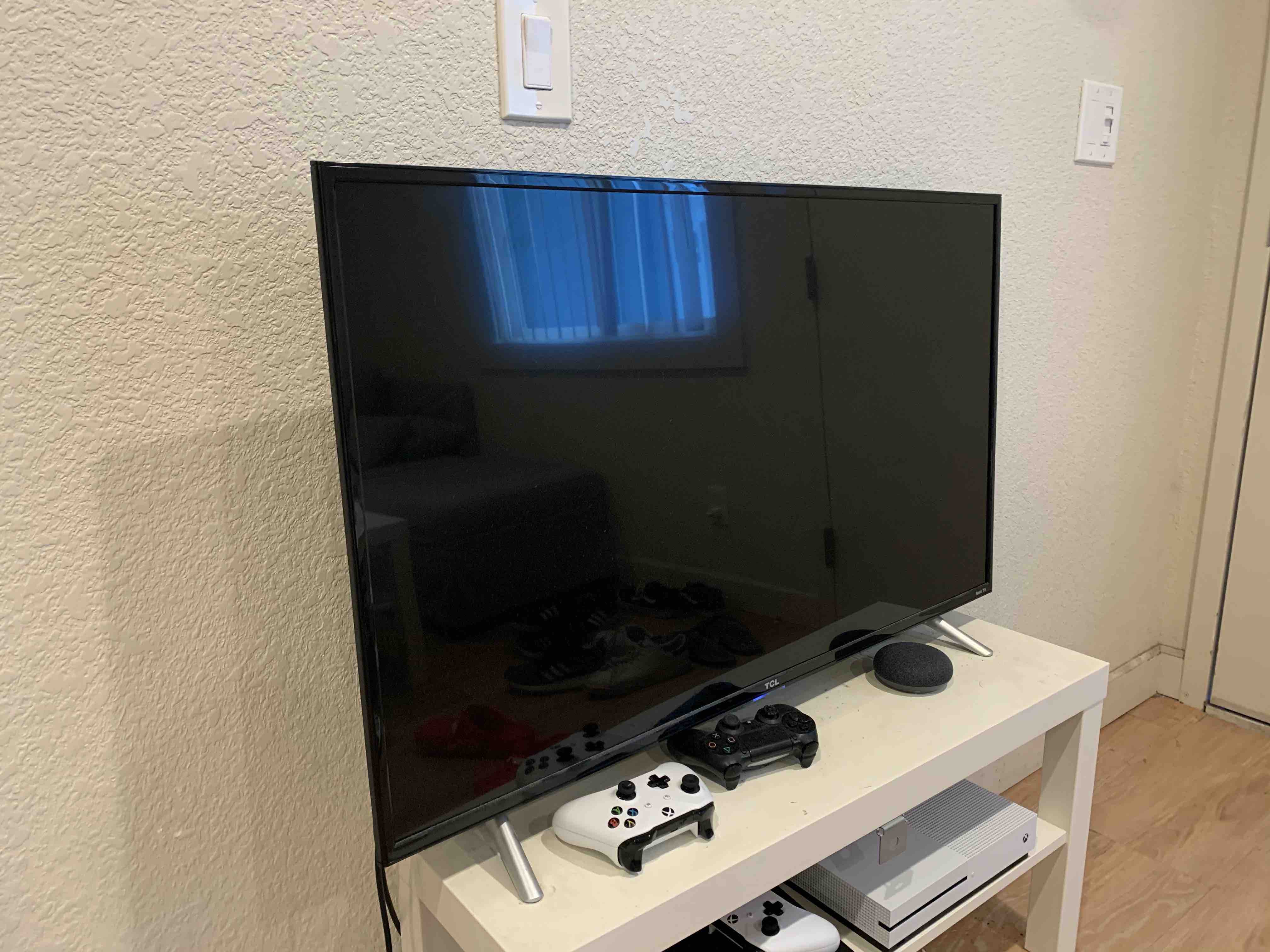
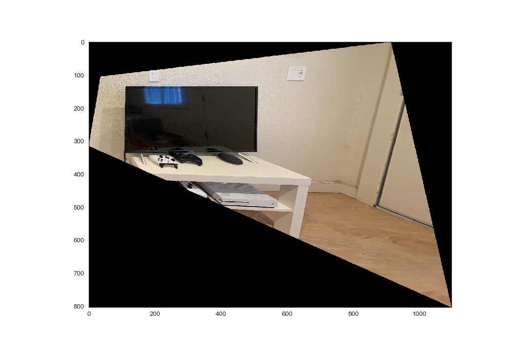
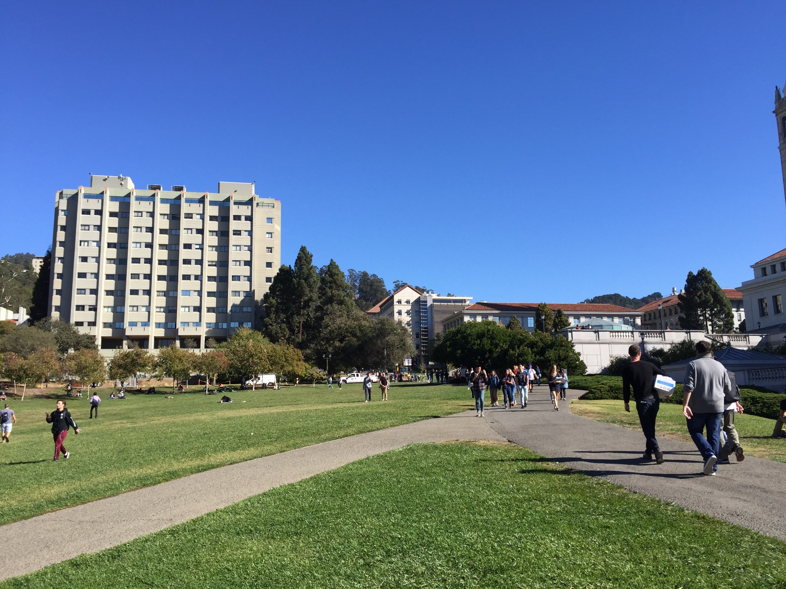
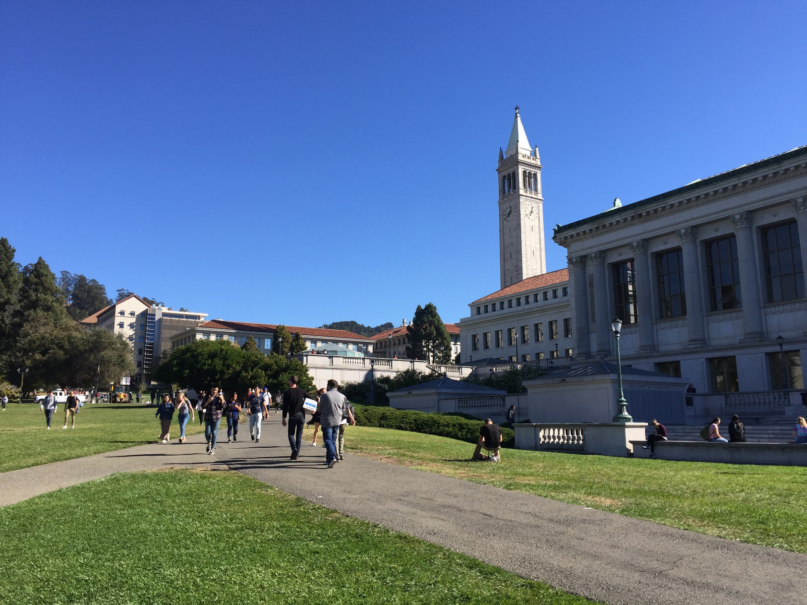
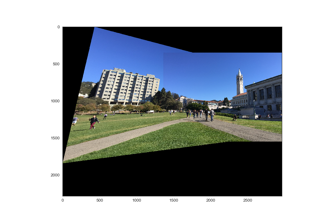
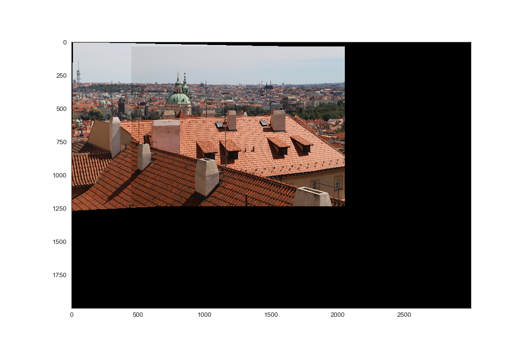
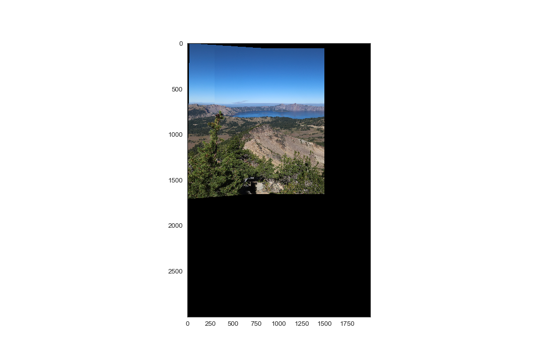
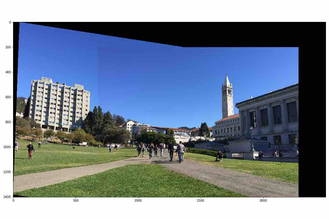
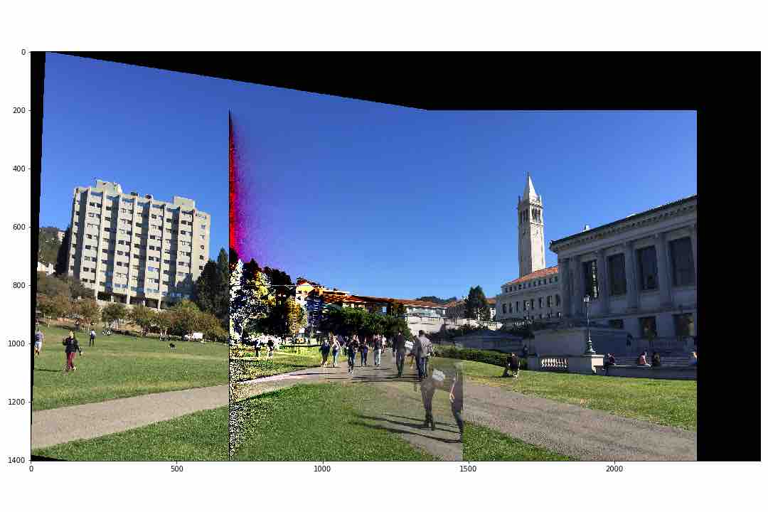
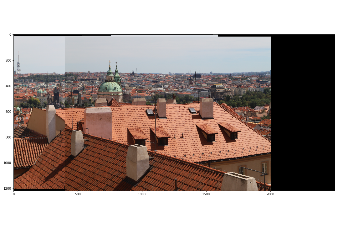
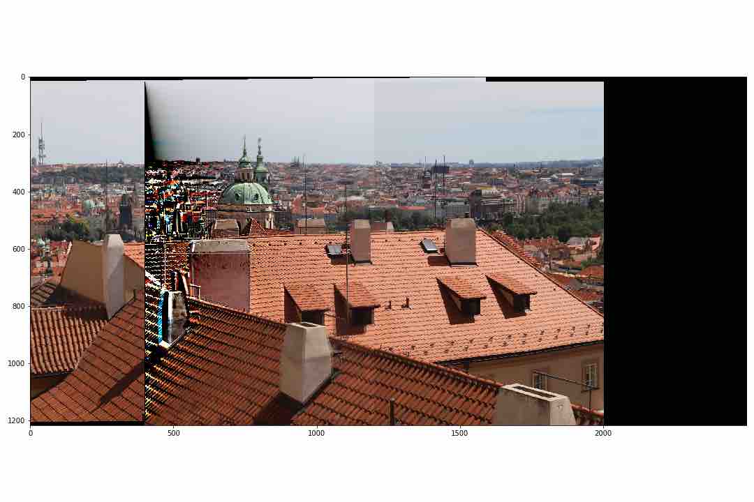
In this section we demonstrate the ability to recover homographies to warp an image to the perspective of another image, and blend both images together to create a panorama, or wider field of view of the subject matter. As before, this procedure begins with selecting correspondences between the two images to compute the homography matrix H. Next, we determine a larger bounding box to be able to display the warped image, and the second image. This is done by computing the dot product between H and a 3x4 matrix C containing the coordinates of the corners of the original, unwarped image:

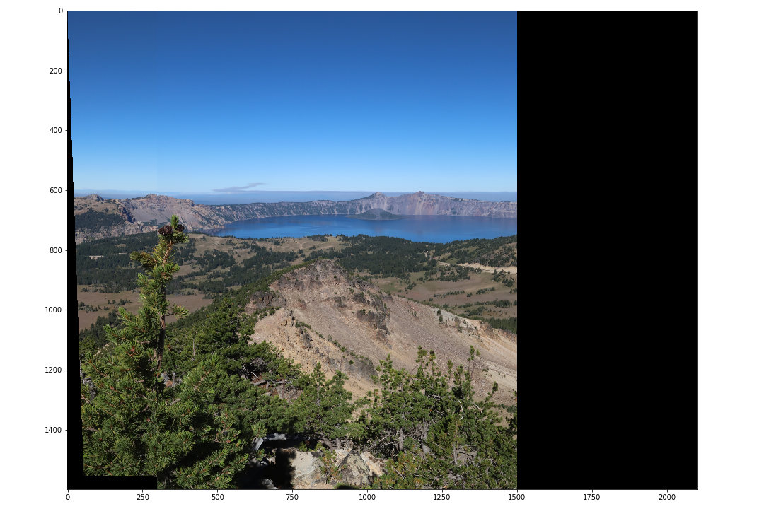
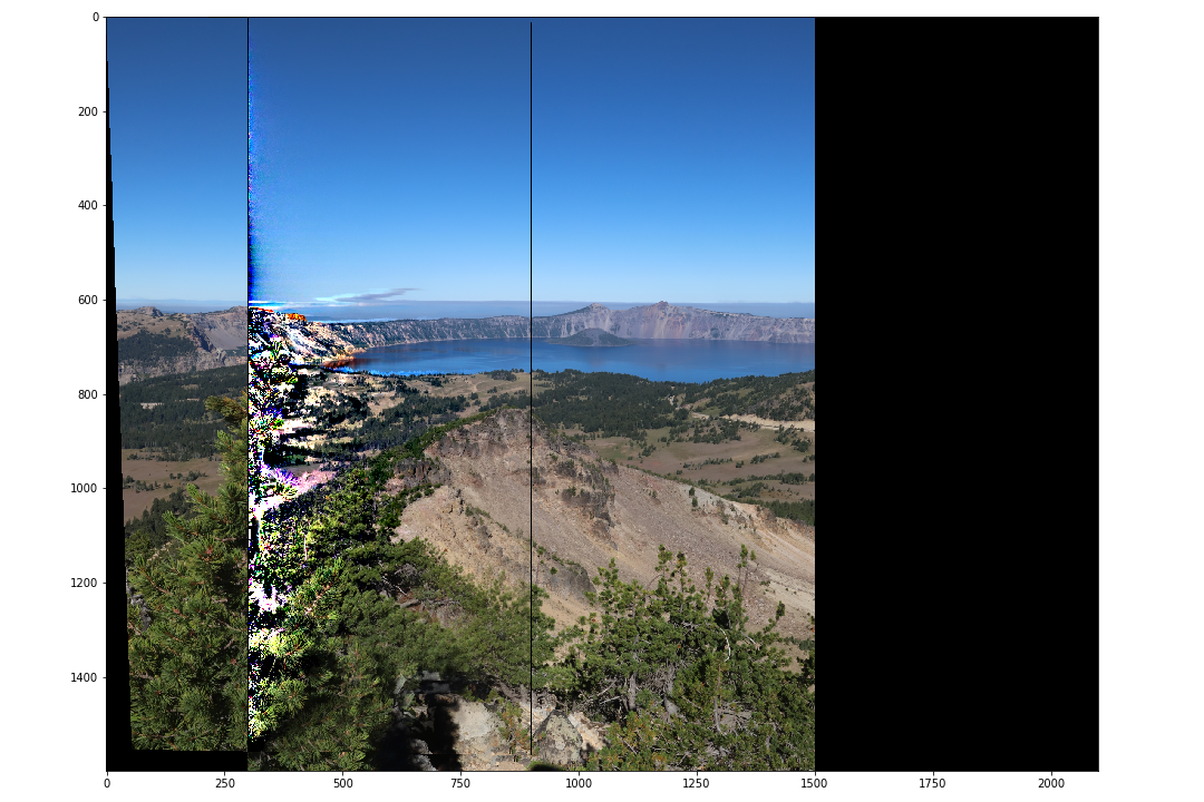
C = [\begin{matrix} x_{0} & x_{1} & x_{2} & x_{3} \\ y_{0} & y_{1} & y_{2} & y_{3} \\ 1 & 1 & 1 & 1 \end{matrix}]

Using the dimensions resulting from the aforementioned dot product, a blank canvas is formed, in which the warped image is first placed, and then the second, unwarped image is placed on top, overwriting any overlapping pixels. In the next part of the project, we'll implement a better method to blend the two images together. The result of this part is shown here:

Part B: Feature Matching and Autostitching

Overview

In part B of this project, we aim to automate the tedious task of manually selecting correspondence points by automatically detecting feature matches betweeen two given images. To that end, we implement a simplified version of the algorithm described in "Multi-Image Matching using Multi-Scale Oriented Patches" by Brown et al.

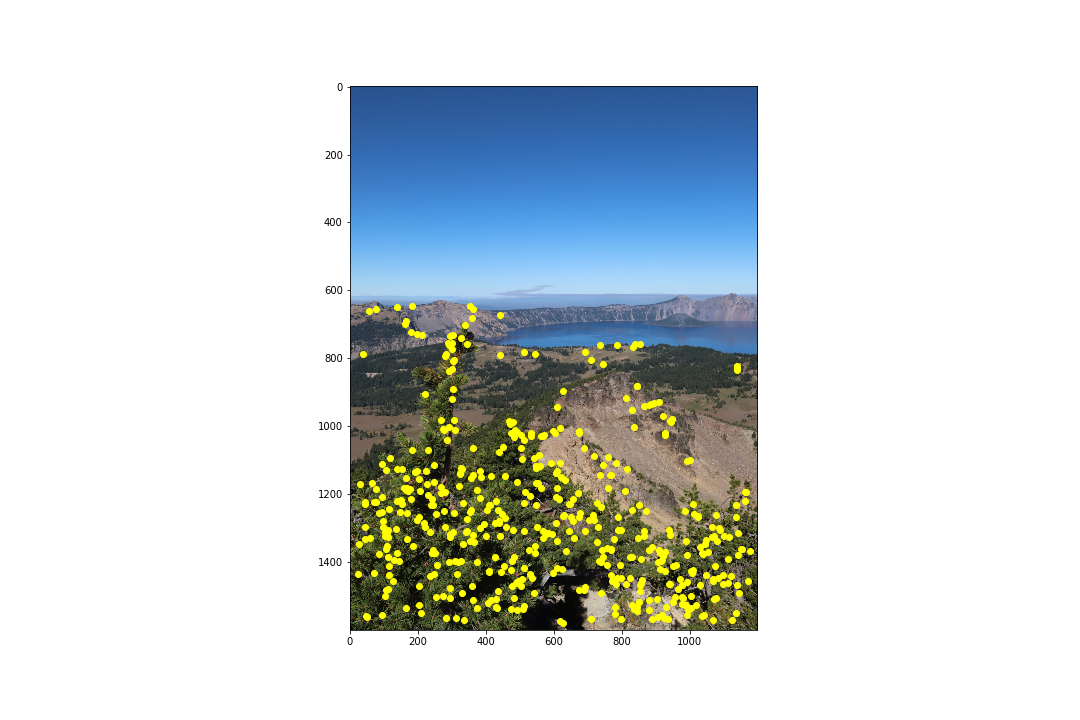
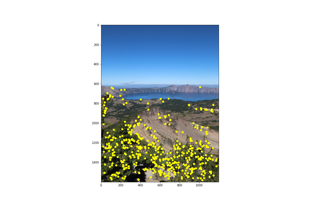
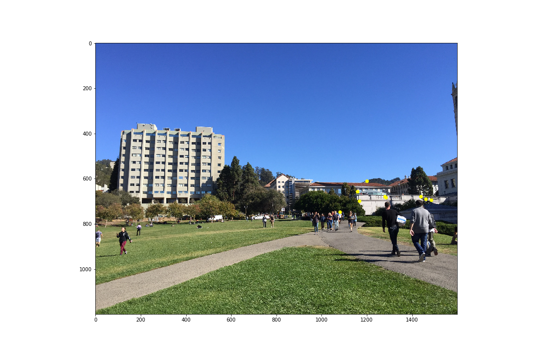
Harris Corners

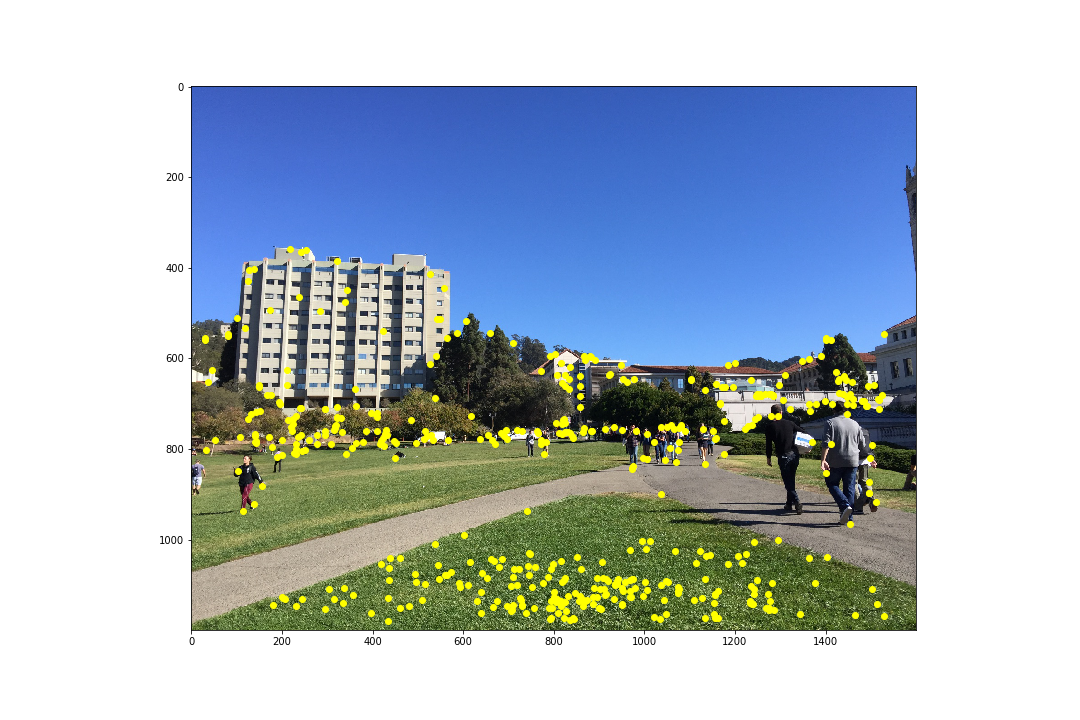
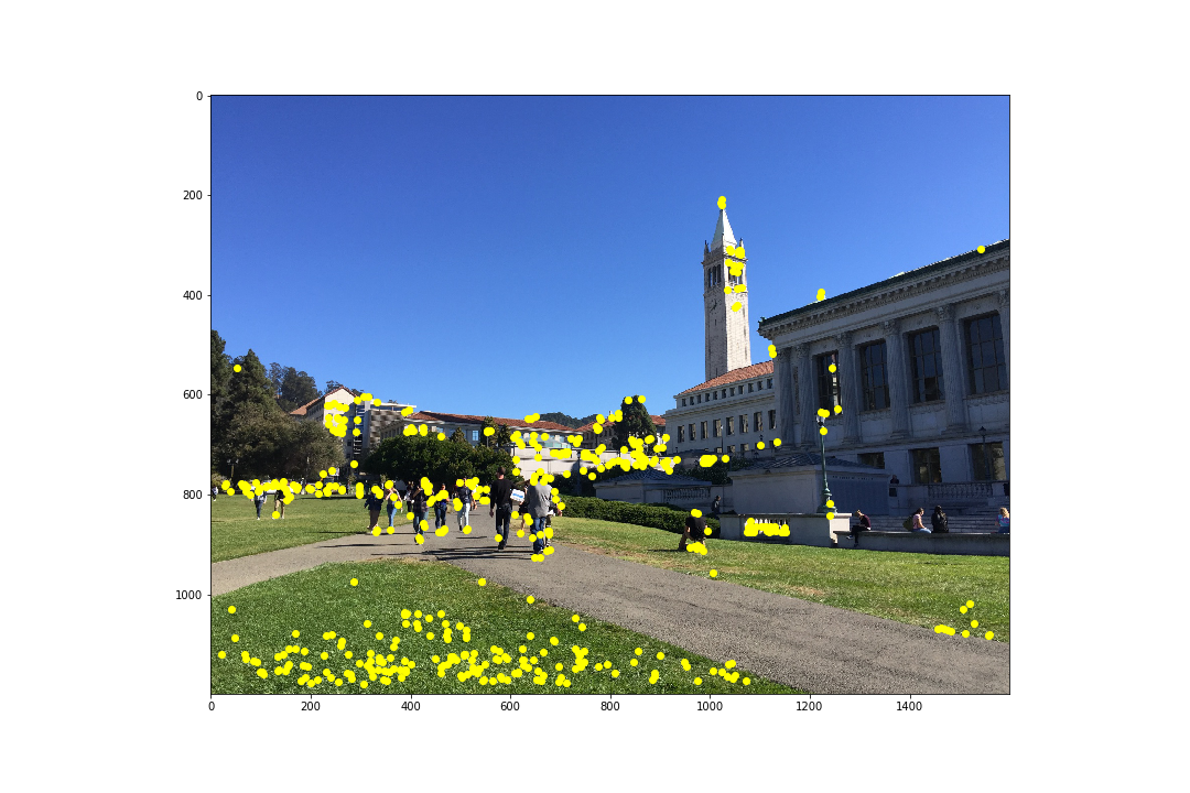
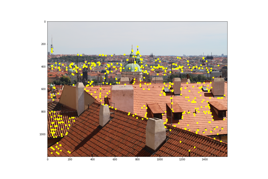
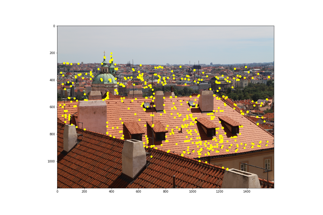
Before finding feature matches between images, we need potential points of interests. These can be obtained using the Harris Corner Detector algorithm which finds corners in an image. I used the code provided to us in harris.py but within get_harris_corners I used corner_peak instead of peak_local_max as it returned far less random points of interest. The following pairs of images are the points of interest that the Harris Corner Detector algorithm found:

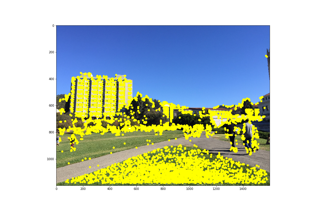
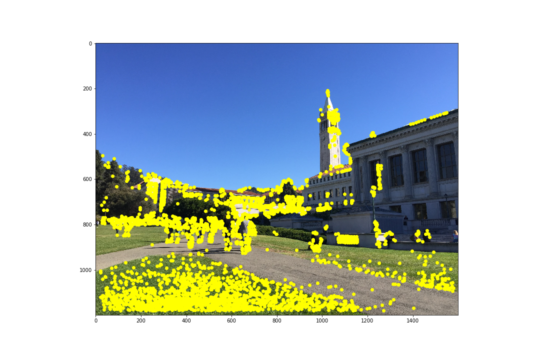
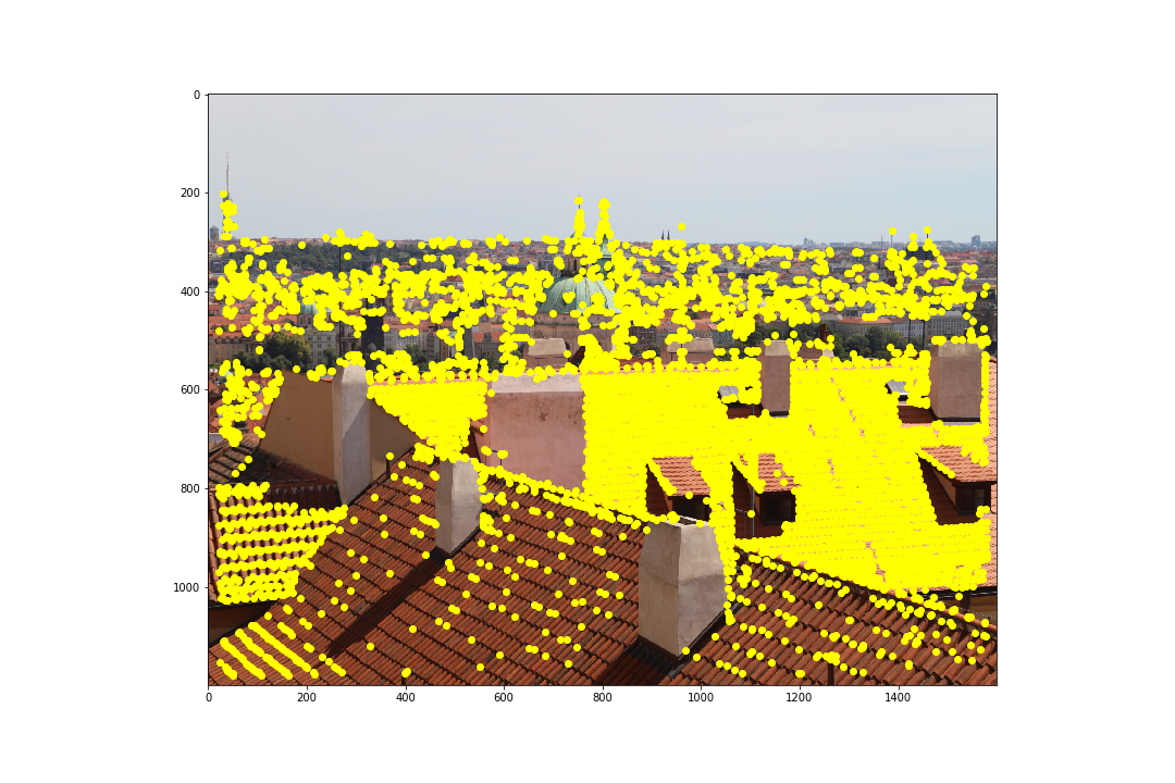
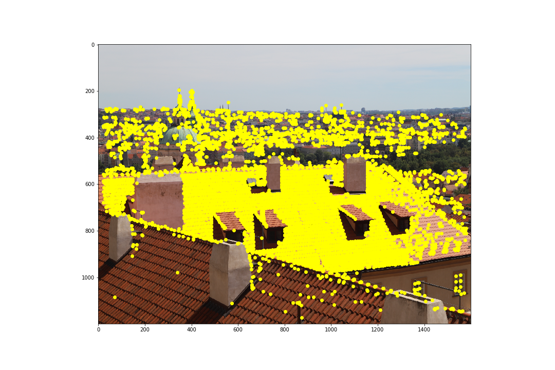
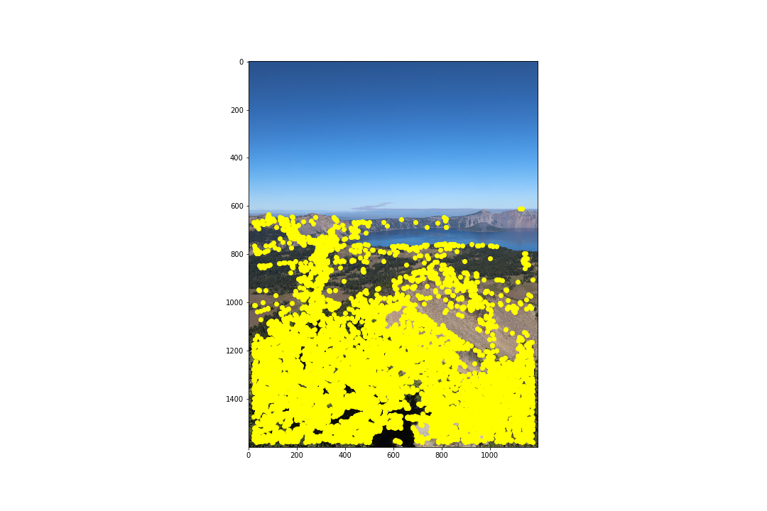
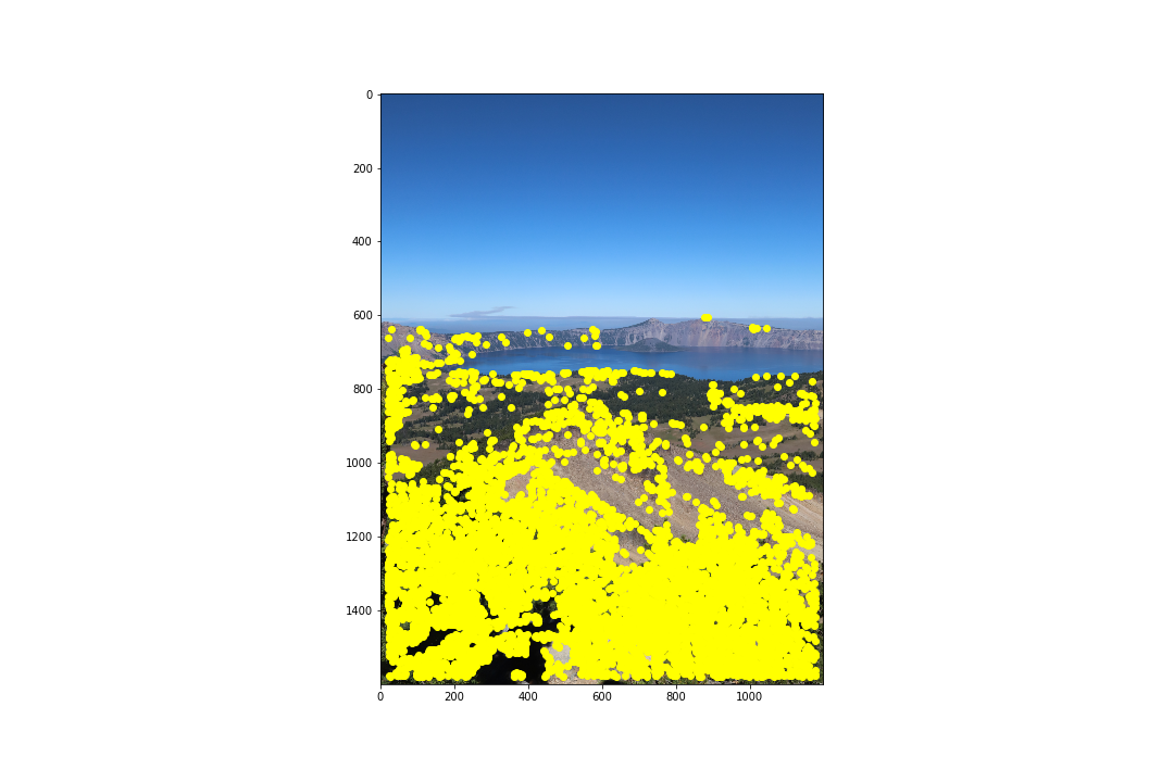
As we can see, though this detects points of interests, there are far too many points to efficiently compute a homography. Next, we aim to reduce these by using Adaptive Non-Maximal Suppression (ANMS).

Adaptive Non-Maximal Suppression

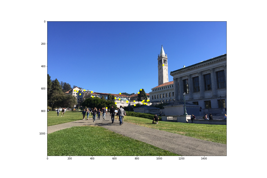
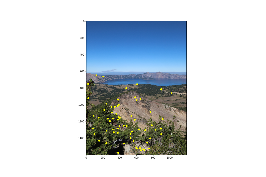
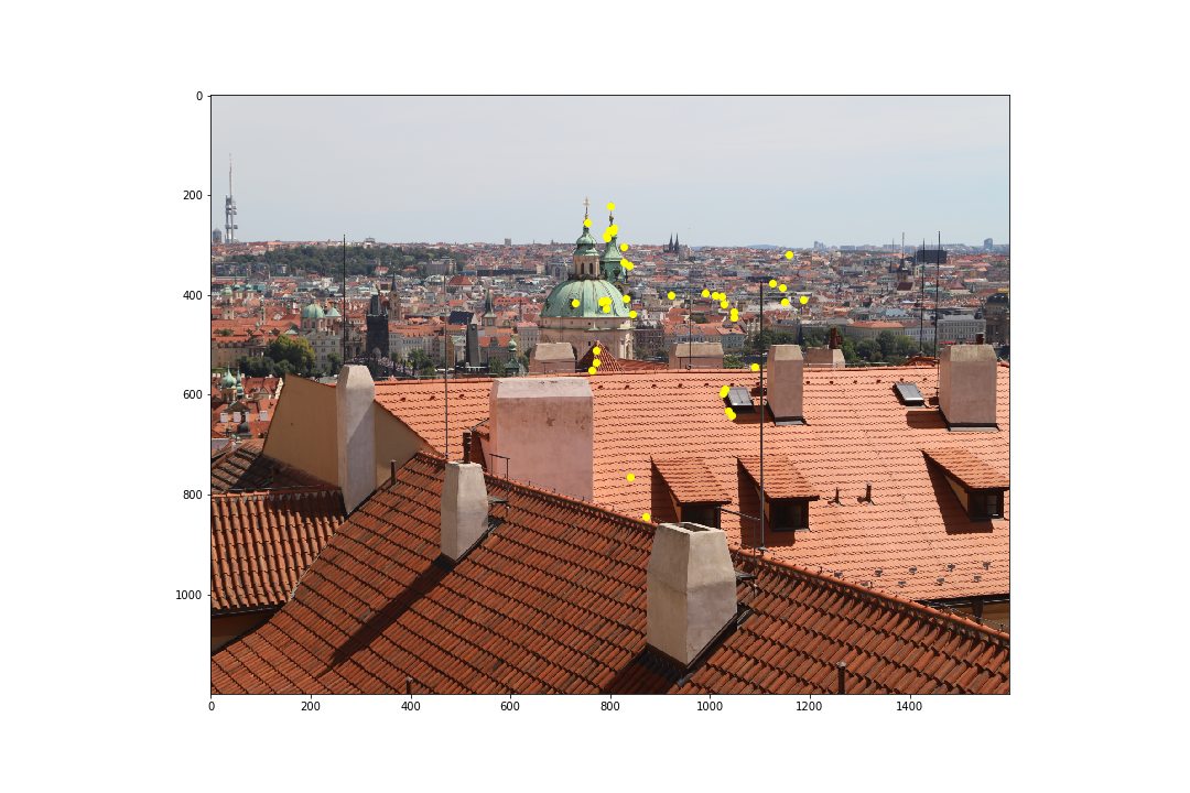
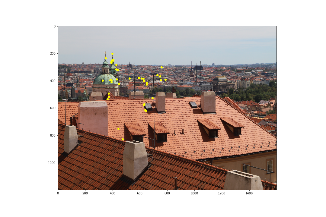
As the Brown et al. paper describes, the computational cost of matching is superlinear in the number of interest points, so it is desirable to restrict the maximum number of interest points in each image. Additionally, it is important that the interest points are spatially well distributed over the image. ANMS selects points with the largest values of $r_{i}$ : the minimum suppression radius of a point $x_{i}$ . Brown et al. presents the following algorithm:

r_{i} = min_{j} | x_{i} - x_{j} |, s.t. f (x_{i}) < c_{robust} f (x_{j}), x_{j} \in I

$I$ is the set of all interest points, and $f (x)$ represents the corner response from the Harris Corner Detector algorithm for a point $x$ . Brown et al. found a value of $c_{robust} = 0.9$ to work well. We keep the top 500 points. The results on our images is as follows:

Already from this we can begin to see some clustering of points of interests, so next we can perform feature matching.

Feature Descriptor Extraction

With this limited set of 500 interest points, we perform feature descriptor extraction by extracting a 40x40 patch centered about each coordinate. This patch is downsampled to 8x8 in order to reduce high frequency signals. As per Brown et al., the patches are normalized in bias and gain by subtracting by their mean and dividing by their standard deviation. This ensures the features are invariant to affine changes in intensity (i.e. bias and gain). Using these descriptor patches, we can match features by performing a nearest-neighbor search between the patches in one image to the other image.

Feature Matching

The Brown et al. paper outlines feature matching as a nearest neighbor search, which I've implemented as the sum of squared differences (SSD) between the patches in one image to the other. In order to determine a feature match, the Lowe ratio test is used:

1 - N N / 2 - N N < thresh

where I found a value of $thresh=0.65$ to provide a sufficient number of matches. The results of feature matching are as follows:

As we can see, feature matching did a good job pruning the points to find matches, but still keeping them fairly spread out over the whole image. However, some correspondence points still don't match up perfectly between the two images. Since the homography matrix is computed using least-squares, the result is highly sensitive to outliers, and so we must remove outliers. To remove outliers, we look towards RANSAC (RAndom SAmple Consensus)

RANSAC

RANSAC runs over several iterations, wherein it selects 4 potential matches at random from the first image, and computes an exact homography. Then, all points from the first image are warped to the second image, and we compute the SSD error between these warped points and the actual points in the second image. Inliers are defined as points with an SSD error within a certain threshold, and RANSAC keeps track of the largest set of inliers and returns that. In my case, I found 10,000 iterations and a threshold of 5 to work well. The results of RANSAC are as follows:

As we can see, RANSAC removed outliers that were present in the correspondences.

Automatic Stitching

I performed automatic stitching in the following way:

Create a blank canvas of size (im_1_height + pad_canvas_y, im_1_width + pad_canvas_y)
Place the warped im_2 image at canvas[:im_2_warped_height, :im_2_warped_width]
Place im_1 image at canvas[(im_1_height+im_2_warped_height)/2-im_1_height+pady:(im_1_height+im_2_warped_height)/2+pady, canvas_width-im_1_width+padx:canvas_width+padx]
Adjust padx and pady accordingly to line up images

Blending

I performed blending on im_1 while placing it into the canvas. Any points on the canvas where im_1 would go that were originally blank (black; 0) were simply set to that pixel in im_1. However, points that overlapped with the pre-existing pixels from placing im_2_warped were blended using a ratio of the distance a point was from the center of im_1:

r*P1+(1-r)P2

Moving away from the center, the ratio r would decrease to 0, meaning distant points from the center of im_1 that overlapped with im_2 would be less visible compared to the im_2 pixels at that coordinate. This resulted in some strange artefacting towards the edges of im_1 as shown in Results.

Results

The left column shows the results from manual cropping, the middle column shows the results from automatic cropping but no blending, and the right column shows the results from automatic cropping and blending.

Both the manual and automatically stitched images look similar, but the homography for the manual images seems to perform slightly better. This is due to having more point correspondences (20) in most cases, and no need to rely on a robust outlier detection algorithm. To be able to skip the tedious task of selecting correspondence points manually, the small differences in the homographies are insignificant.

Final Thoughts

The coolest thing I've learned from this part of the project is the formulation of the linear algebra behind computing the homography matrix. Coding an implementation to solve for the matrix helped me understand how the perspective warp takes place, moving the pixels from the source locations to destination locations in the new perspective. Also, this once again gave me an appreciation for the simplicity and capability of least squares.

References

Images taken from Shivam Parikh's "course provided images", and Andrew Campbell's class project from Fall 2018.