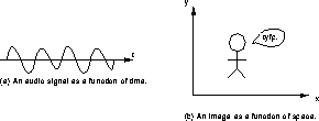
Figure 1: Signals as a function of time and space.
EECS20: Introduction to Real-Time Digital Systems
Lab13: Image Processing
EECS20: Introduction to Real-Time Digital Systems
©1996 Regents of the University of California.
By K. H. Chiang, William T. Huang, Brian L. Evans.
URL: http://www-inst.eecs.berkeley.edu/~ee20
News: ucb.class.ee20
Resist printing this out from a web browser; you will get two huge images killing the printer. Print out the Postscript version instead.
In previous labs, we worked with one-dimensional signals, which were good for representing sound. Extending the notion of a one-dimensional signal to two dimensions lets us deal with images.
With audio, we could represent a signal as a sum of appropriately scaled and phase-shifted sinusoids. Since the audio signals were taken against time, as in Figure 1(a), ``frequency'' meant a variation in time.

Figure 1: Signals as a function of time and space.
With images, we could also represent a signal as a sum of appropriately scaled
and phase-shifted sinusoids. However, images are functions of space, as
in Figure 1(b). So ``frequency'' means a spatial variation instead,
and since we have two dimensions in space, we allow a spatial variation in the
 direction and a spatial variation in the
  direction.
You will need to familiarize yourself with a number of commands in order to perform image processing in Matlab.
Station 1 is equipped with a camera that can be used to grab single frames.
The capture program is in the Windows group ``Video for Windows 1.1''.
Unfortunately, the only format that the capture program understands is
.dlb. A conversion program should then be used to convert .dlb
format to one of the following: .bmp, .gif, .hdf,
.pcx, .tiff, or .xwd, since these formats are those that
Matlab understands.
The following sequence of commands reads a file khc.gif, converts it to
a grayscale image, and displays it with 256 gray levels. We will not be
dealing with color images.
>> [I,map] = gifread('khc.gif');
>> J = ind2gray(I,map);
>> imshow(J,256)
>> colorbar
The first command reads the file into a matrix I. Each element of
I represents a pixel in the image. The matrix map holds the
colormap of the image; for GIFs, the colormap is usually 256 colors, where a
color is a three element vector that represents some amount of three
primary colors, usually red, green, or blue, but sometimes cyan, yellow, and
magenta. Anyway, each pixel in I is an integer indexing into the
colormap. Together, I and map are called an indexed image.
The second command converts the indexed image into a grayscale image; grayscale images are sometimes termed intensity images. The third command displays that image with 256 gray levels, while the final command adds a somewhat useful bar showing the gray levels to the right of the image.
In lab 6, we used the Matlab fft command to determine the frequency
domain representation of a given signal. The fft2 command extends
fft to two-dimensional signals.
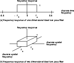
As we saw with audio, we can filter a signal to recover its low frequency components. In one dimension, the ideal lowpass filter has a frequency response as in Figure 2(a).

Figure 2: Ideal lowpass filter frequency responses.
In two dimensions, the ideal LPF has a response as in Figure 2(b).
One of the more popular lowpass filters is the Gaussian, as in Figure 3,
which has the interesting property that its frequency response is also a
Gaussian. In Matlab, a Gaussian can be generated by using the fspecial
command; assuming that we have a grayscale image J, the following
commands will generate a Gaussian and filter J with that Gaussian:
>> g = fspecial('gaussian', n, sigma);
>> K = filter2(g, J);
>> imshow(K, 256);
The argument n sets the filter size; if n were 10, the resulting
filter would be 10x10 in size. sigma sets the width of the Gaussian in
pixels; the smaller the value, the higher the cutoff frequency.
We saw that a one dimensional signal  could be quantized by normalizing and
then performing:
>> floor(x*2^n) / 2^n
Two-dimensional signals can also be quantized. In the case of grayscale images, since the values all lie in the interval [0,1], normalization is unnecessary.
With audio, excessive quantization can be thought of as introducing signal-dependent noise. With images, excessive quantization introduces false contours and lines in the images.
In the medical community, image processing is useful in bringing out features in X-rays that would otherwise be obscured. Because different materials absorb X-rays at different rates, the intensity of a given pixel in the resulting grayscale image is indicative of the material at that spatial location.
Thus, certain features of given X-ray images can be enhanced by noting the range of intensities of the desired features, and then brightening the desired intensities, darkening the undesired ones, or some combination of both.
Sometimes we'd like to reduce the size of a given image, so that it takes up less storage space. This also allows us to consume less bandwidth when sending that image over a communications channel.
One of the more popular image storage formats is JPEG. JPEG employs the discrete cosine transform to perform lossy compression. The transform exhibits good energy compaction properties; energies that are largely evenly distributed in the signal domain usually end up in the lower frequency components in the frequency domain. This permits us to throw away the components corresponding to the higher frequencies, since they contain significantly less information, and the degradation in picture quality is not too noticeable.
Compression can also be performed by quantizing an image and then looking at the bit planes of that image. For instance, if an image is quantized to eight bits, there are eight bit planes, or eight black and white images. If the bit planes corresponding to the lower bits exhibit no structure [i.e. if they look like noise], then the entire bit plane can be thrown away with little degradation.
One more way compression can be performed is by plaids. If an image is treated
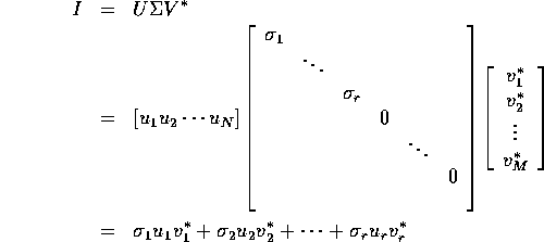
as a matrix, a computationally expensive linear algebra technique called singular value decomposition can be done. If  is an
is an  by
by  image, the
SVD gives

 is a rectangular matrix of size
  by
by  , with nonzero elements only
on its main diagonal; let us suppose that these elements are arranged in
decreasing order, and the after
  of these elements, the rest are zero. The
SVD gives
  and
and  which are unitary, of size
  by
by  and
and  by
by  respectively. If
  is written in terms of its columns and
  in terms of
its rows, then:

Each of the  terms in the preceding sum are called plaids, since they
resemble plaid cloth patterns. Anyway, not all
  terms in the preceding sum
are useful. After some point, the associated
  , where
  , are so small that they can be neglected. This is the basis of the plaid
demonstration on the eecs20 web site.
 by subtracting a Gaussian filter
  of width
 from a Gaussian filter
  of width
  , with
  [so
[so  ]. Filter your images with the constructed filter
 . Experiment with different values for
  and
and  . Is
. Is
 a lowpass, highpass, allpass, bandpass, or bandstop filter? Verify your
answer by using the following Matlab command:
>> surf(fftshift(abs(fft2(g3))));
![[medimage1]](../c20468-2.gif)
![[medimage2]](../c20504-2.gif) Store these images by right-clicking on them, and using the ``save this image
as...'' option. Images courtesy of the National Center for Health Statistics,
Centers for Disease Control
Store these images by right-clicking on them, and using the ``save this image
as...'' option. Images courtesy of the National Center for Health Statistics,
Centers for Disease Control >> dctdemoNow you have a feel for how JPEG works.
svd:
>> [U,S,V] = svd(I);Note that the
V returned by Matlab is not  . Read the
associated help text for the
 svd command for further details.