In this project, we will be doing texture transfer with image quilting. What this algorithm does is that it allows you to take a given texture and expand it to a larger area
or a larger image. This has a lot of applications and can be used for embedding faces or other content within a texture, or for filling in missing parts of an image or for editing objects
out of an image. We will proceed with various methods of image quilting, demonstrating how the method has changed and gotten better each time.
All code for this project can be found at this Colab Notebook here
The drive folder for this data can be found here .
Expanding a Texture
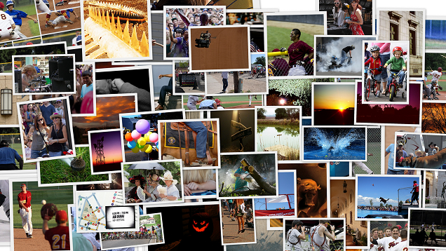
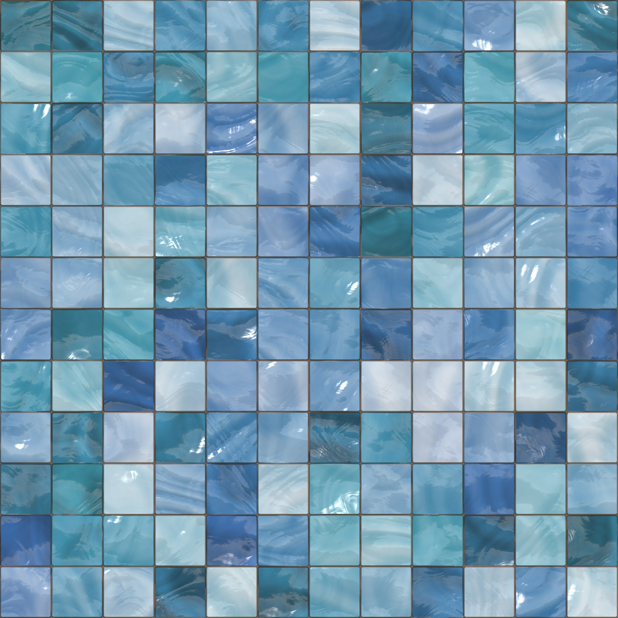
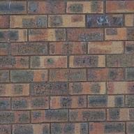
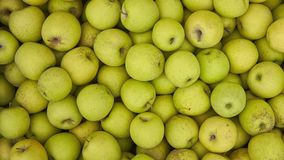
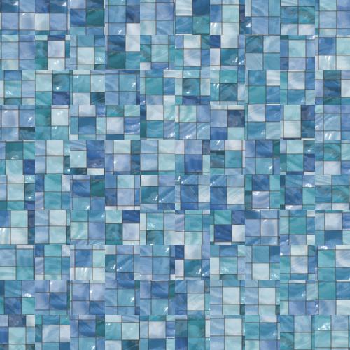
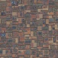
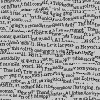
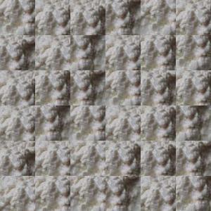
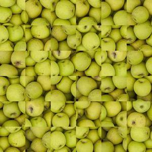
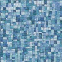
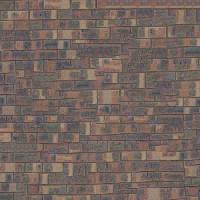
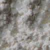
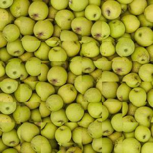
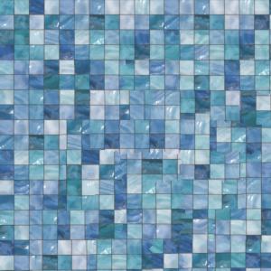
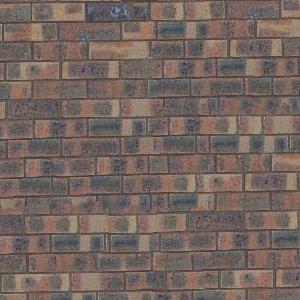
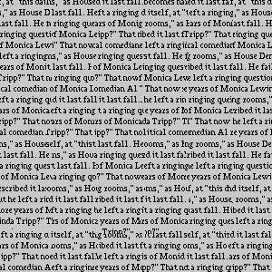
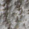
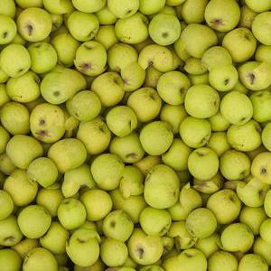
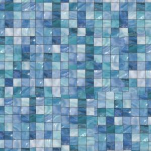
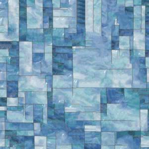
The idea of this is to take a texture and expand it to a larger image so it looks natural. Examples of textures can be seen below:
We want to expand this texture to fill an arbitrary $ M \times N$ image.
Method 1: Random Quilting
This method is by far the easiest to implement but yields the worst results. The algorithm divides the output size into square patch sizes. We then sample
these patch sizes randomly from our texture, and glue them together. We can see the results below:
Our biggest issue is the fact that the colors don't line up and there are artifaces and lines present that make the texture look choppy. We will
investigate ways of tweaking the algorithm to make this better.
Method 2: Choosing Smarter Samples
We keep our iterative sampling subroutine from the previous method, but we modify how we choose our patch. First, we ensure patches have some overlap
between each other. That is the patch on the top left is chosen at random, but each subsequent patch will have some horizontal or vertical overlap with
the previous patches. We will use this horizontal and vertical overlap to our advantage.
The first thing we do is that we choose the top left sample at random. We then proced to the next empty square that overlaps horizontally with the first patch.
We take this image and compute a mask of ones and zeros where the overlap is. Then, we want to determine for each subpatch within the texture, we determine which one
is closest to overlapping region by taking the sum of squared distances between them. This metric will be called the cost of the patch. We speed this up by breaking the SSD computation into convolutions.
Finally randomly sample a patch whose cost is within $(1 + tol)$ of the minimum for our image where $tol$ is set to be small.
This method yields much better results as seen below:
Still, there are a lot of artifacts that stem from the horizontal and vertical nature of our patches. In particular, textures without vertical and
horizontal lines still do not look natural.
Method 3: Seam Finding
We now incorporate seam finding into our algorithm to joint two candidate patches together. Before, we would simply take a chosen patch and overlay the image
with that patch. This, however created unwanted artifacts and lines. From the SSD error, we know that the images are close enough on the overlapping regions. Thus
in order to merge the images together, we compute the SSD only on that patch and find a seam through the patch that determines the lowest energy cost.
For horizontally overlapping regions, a seam is a path from the top of the overlapping region to the bottom of the overlapping region with the lowest cost per pixel
from top to bottom. Seams can move from one pixel to the one directly below it or diagonally to the left or right. For vertically overlapping patches, we simply transposed the image and applied the horizontal algorithm to determine the seam.
Once we did that we transposed it back. To calculate this path, we use dynammic programming.
Here is the seam carving result on a real error patch. The two patches are shown below.
The first image below describes the patches error over the overlapping region. The second image is the seam mask that results from the algorithm. The white is where
the first image should be overlayed and the dark is where the chosen sample should be layed.
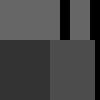
To illustrate the algorithm more clearly, I created test error patches that really drive home the point of this algorithm. Here are two sample error patches where the darker the color, the lower the energy.
The first image has a clear path on the right. The second, however does not it only goes down partially. Here are the results of seam finding on these error patches:
This demonstrates that the dynammic programming approach to this problem is able to accurately find seams from the top all the way down of the lowest cost. Once we had
the seam masks for vertical and horizontal we were able to combine them into a single mask to merge the two images together. After that, we
see the following results:
We also see that the patch size for the image matters. For instance, with the blue tiled texture, the difference between a large (left) and small (right) patch size is apparent:
Takeaways
My biggest takeaway for this part is how we built a robust algorithm out of smaller chunks and morphed one problem into the other
in order to solve the problem. I was surprised by the use of a dynammic programming algorithm here, but it is clearly very powerful and very useful.
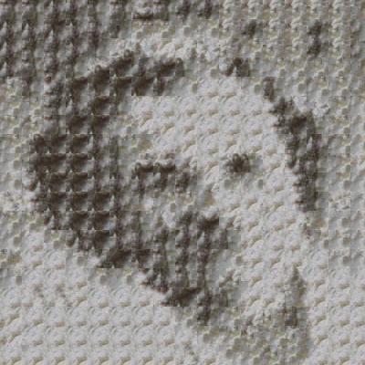
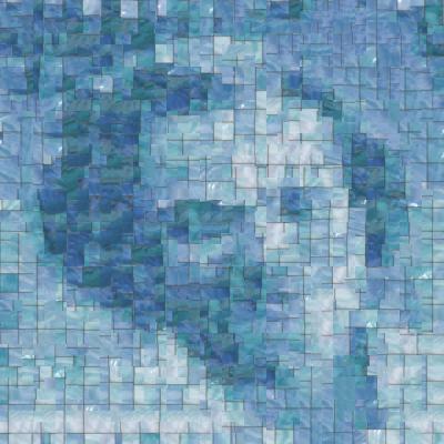
Iterative Texture Transfer (Belles and Whistles)
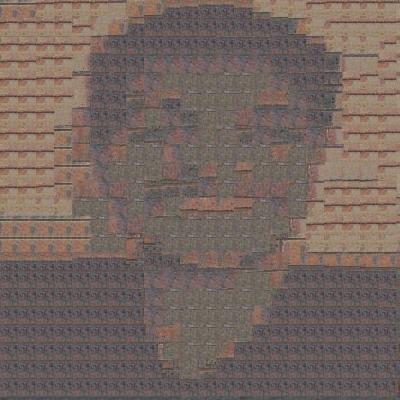
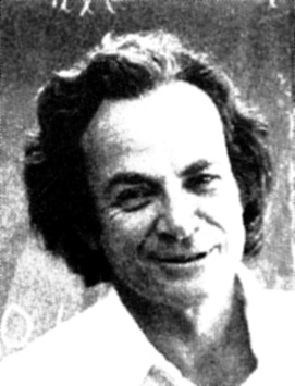
Now that we have solved the problem of texture synthesis, we can use what we have learned to blend an image and a texture together. That is we can
draw a famous image in the style of a texture.
Before, we would create a new image by choosing a sample from a given texture. We would choose the sample by comparing the SSD error between the overlapping regions
of the already generated image and a random image patch. We now also add a term to compare the random image patch to the reference image that we want to transfer over.
To compute this term, we first compute a correspondence map between pixels in one image and pixels in another image. This correspondence map can be anything, but for us,
we chose intensity of the pixel. Other correspondence maps might be blurred intensity or local angle orientation, etc. depending on the use case. The idea being that patches of similar
intensity are good canidates to replace each other. Correspondence cost is simply the ssd error between the correspondence map of the sampled patch and the outputted region.
With this correspondence image, we now proceed iteratively generating an image and modifying it as we go. For each iteration we sample the patch size and a quantity called $\alpha$ which determines
how much weight we put on the correspondence error versus the overlapping error. A high $\alpha$ means a higher weight on overlapping error. At first, we care a lot about capturing the indicated image, so
our patch size is large and our $\alpha$ is low. However as we move through the algorithm, our patch size becomes smaller, and we care more about the details and the overall flow between patches. Thus,
$\alpha$ increases and our patch sizes decreases through each iteration.
Our cost function now becomes
$$ \alpha \cdot (\text{overlap cost}) + (1 - \alpha) \cdot (\text{correspondence cost}) $$
Some other things that were implemented as apart of this algorithm:
Patch errors were normalized before being compared since there was large variance between correspondence error and overlapping error.
Overlap was set to 1/6 of the size of the patch size.