Neural Style Transfer

Introduction

In this project we will be doing style transfer with deep neural networks. This project aims to take the art of one image and transfer its style to the content of another image. We use the features from the VGG_19 batchnormed model to conduct our style transfer. We use this method to reconstruct an image's content and its style from various layers in the neural network. Finally, we combine the two methods to construct an image whose content matches one image, and whose style matches the other. All code for this project can be found at this Colab Notebook here

Creating Loss Functions

The premise of this algorithm is to use a pre-existing neural network, which we define as $N(x)$ that takes in an input image and computes features on each of its individual layers. We want to create loss functions that will take in an arbitrary noisy image and using gradient descent, compute an image whose features match those of a reference image in some sense. This is the premise of content and style loss.

Content Loss

Content loss is very simple. For a given layer $l$, we compute the SSD between the features of the reference image and the features of the input image. The NN network parameters and reference image parameters are static, the only gradients that are computed are that of the input image itself. $$ \mathscr{L}_{\text{Content}}(x, r, l) = SSD(N(x)[l], N(r)[l]) $$ where $r$ is the reference image, $x$ is our noisy image, $l$ is our layer, and $N$ is the neural network function.

Style Loss

Style loss is a bit different. Two images of similar styles will not have the same pixel values at each stage. They will, however have similar correlations between feature maps (or channels) of a given layer. We can think of a layer as $c$ channels worth of ``images'' each with height $h$ and width $w$. Thus, we compute the Gram Matrix $G$ between a layer and itself which will be a $c \times c$ matrix. The gram matrix is such that $G_{i, j}$ is the image at the $i$th channel dot product with the image at the $j$th channel. We then normalize the Gram matrix by dividing by the number of entries ($c \cdot \w \cdot \h$) in the layer. We then define our style loss as the SSD between the gram matrix of the reference, and the one of the input. $$ \mathscr{L}_{\text{Style}}(x, r, l) = SSD(G(N(x)[l]), G(N(r)[l])) $$ Where $G$ is the function that takes in a $c \times (h \times w)$ layer and returns a $c \times c$ matrix.

Final Loss

The final loss function is dependent on how much content vs style we want in a given image. Suppose our content reference is $c$ and our style reference is $s$. We have $\alpha$ and $\beta$ as parameters in our algorithm that determine the amount of content vs style that we need. We also define $C_L$ and $S_L$ as the layers that we wish to compute content and style loss on. Our final loss function is then: $$ \alpha \sum_{l_c \in C_l} \mathscr{L}_{\text{Content}}(x, c, l_c) + \beta \sum_{l_s \in S_l} \mathscr{L}_{\text{Content}}(x, s, l_s) $$ What we now need to do is determine which layers are best for content, and which are best for style.

Running our Final Algorithm

To run our final algorithm, we simply choose values of $\alpha$, $\beta$, $C_l$ and $C_s$ and have the algorithm backpropagate errors onto an image of white noise. Once this is done, the image will turn into a blend of content from one image, and style from the other.

Content and Style Reconstruction

To determine what is best for each layers, we run experiments on the content and style reconstruction of a given image.

Content Reconstruction

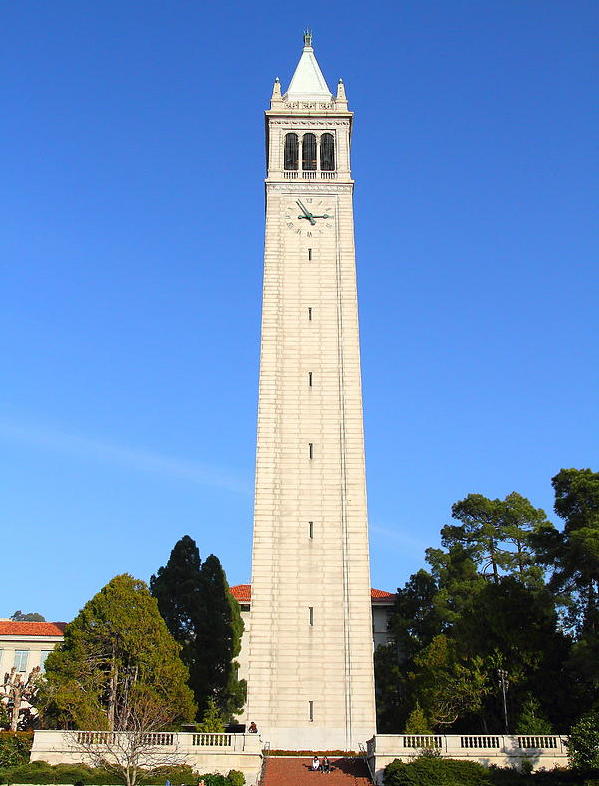
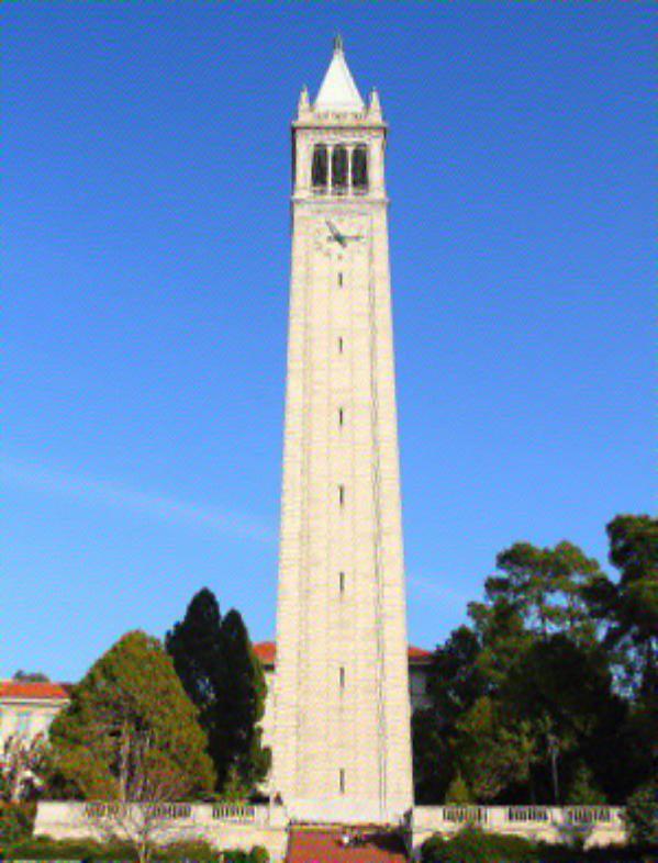
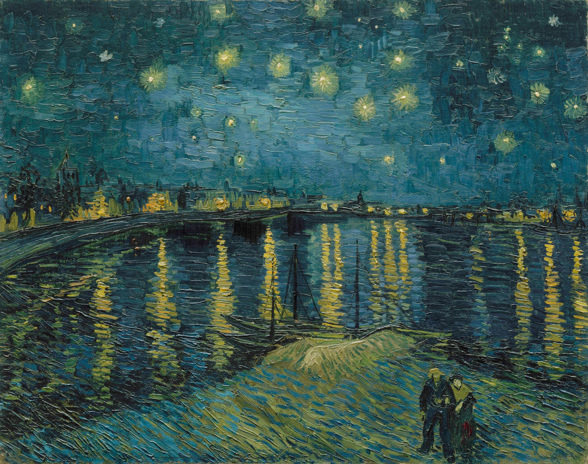
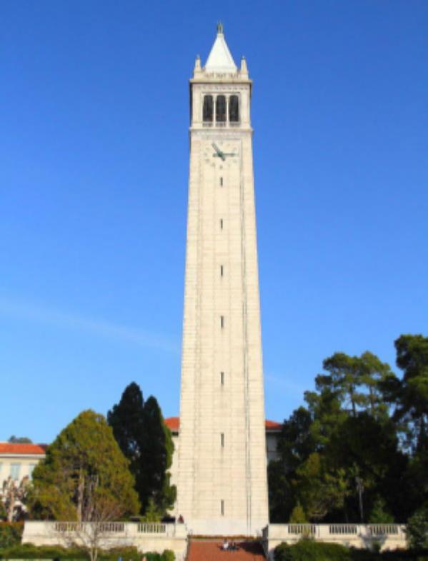
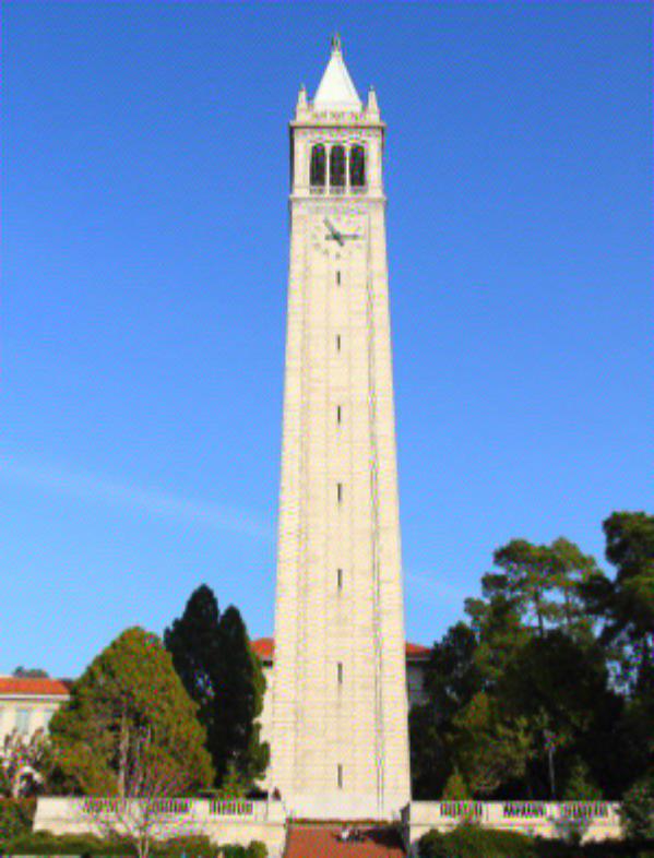
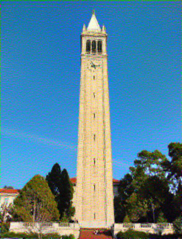
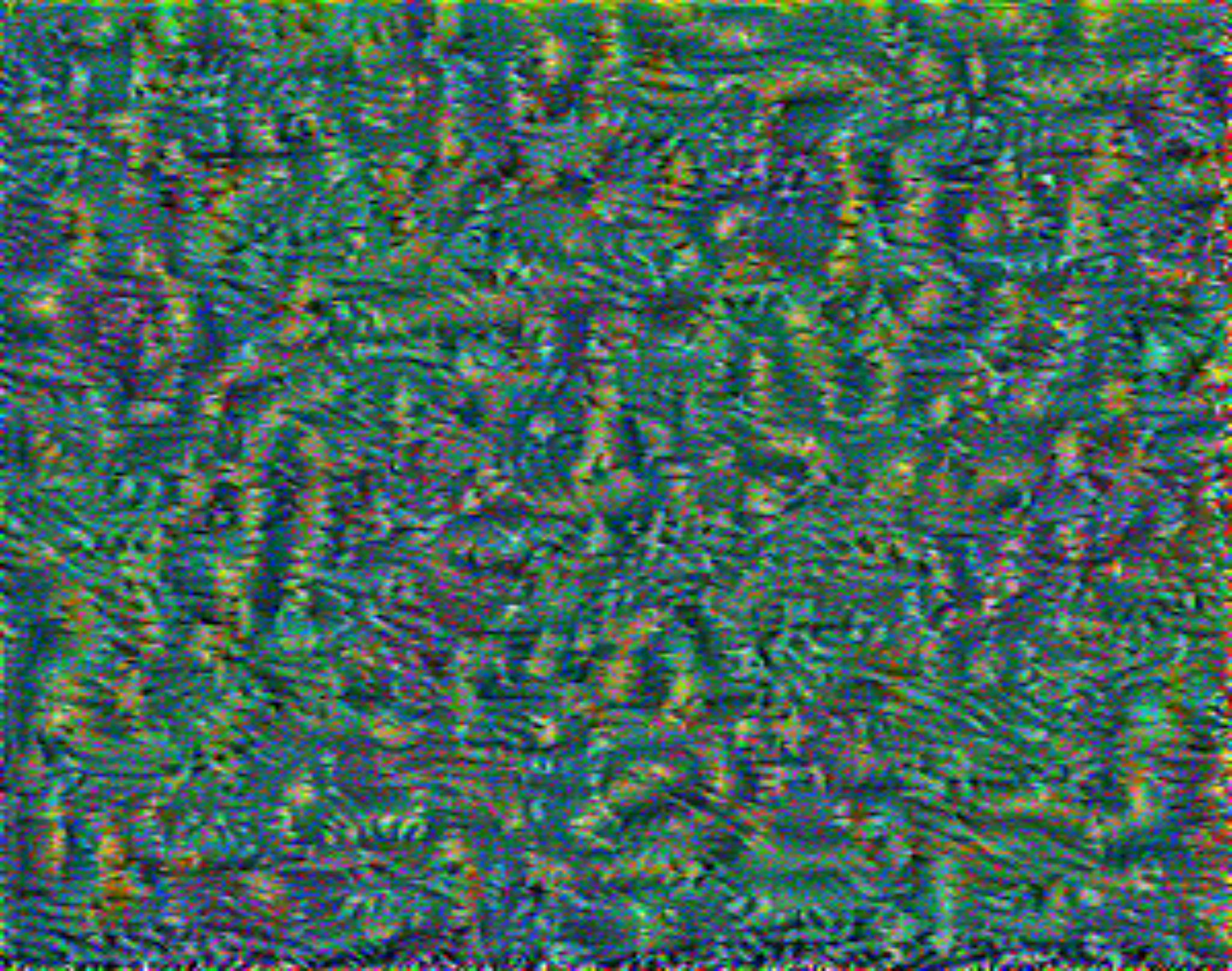
For the given content images we run content reconstruction for a single layer. In this case we set $C_s = \emptyset$ and set $C_l$ to be a single layer and run the algorithm. Original Images: We now show our reconstruction for the first, fourth, sixth and eigth layers. Some takeaways are that content reconstruction is really good even for later layers, and if we want to strip the style away from these images then we should look at later layers where the style starts to break down (hence the more pixely and wavy shapes). It is here where the content will not be as overpowering as the other layers.

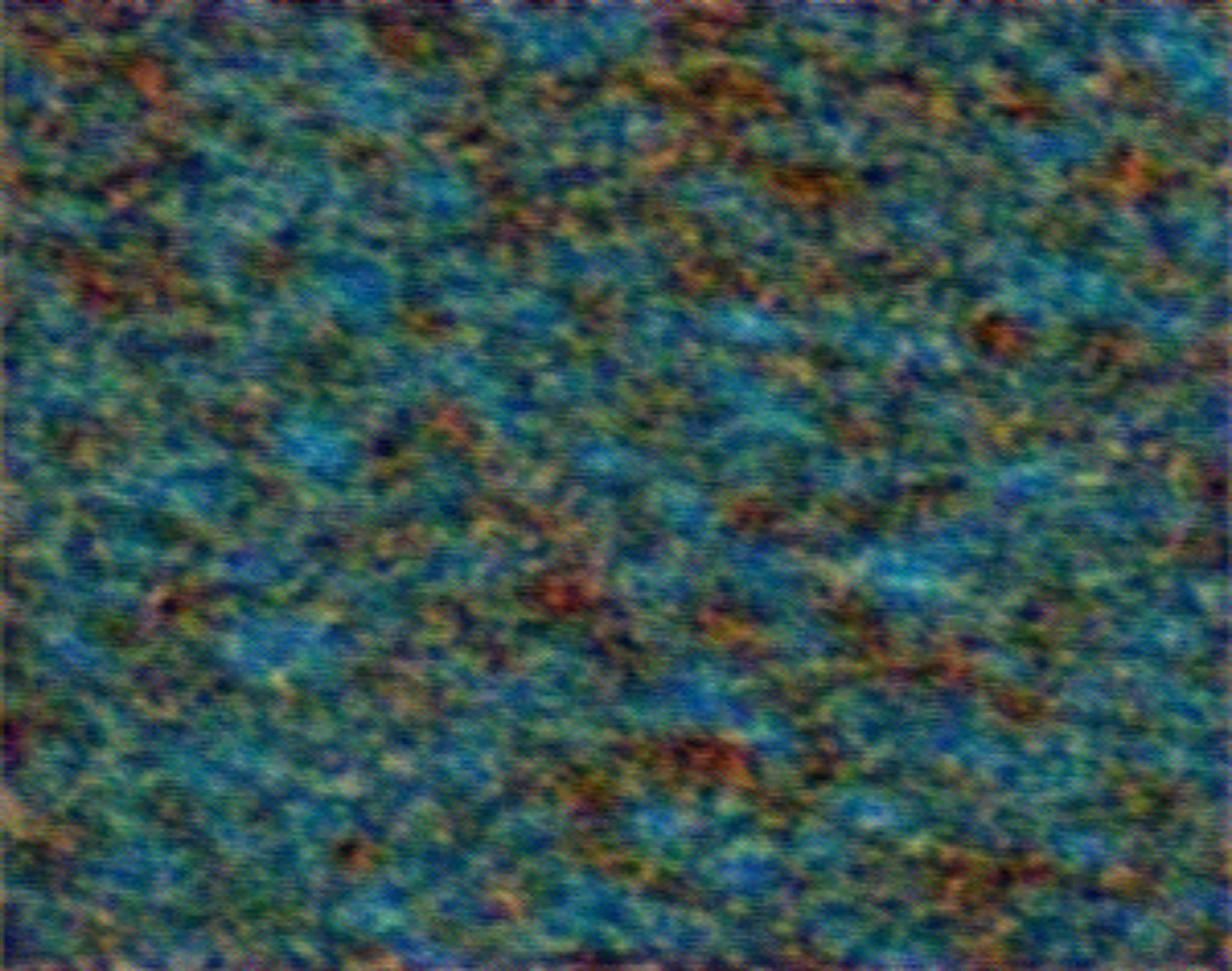
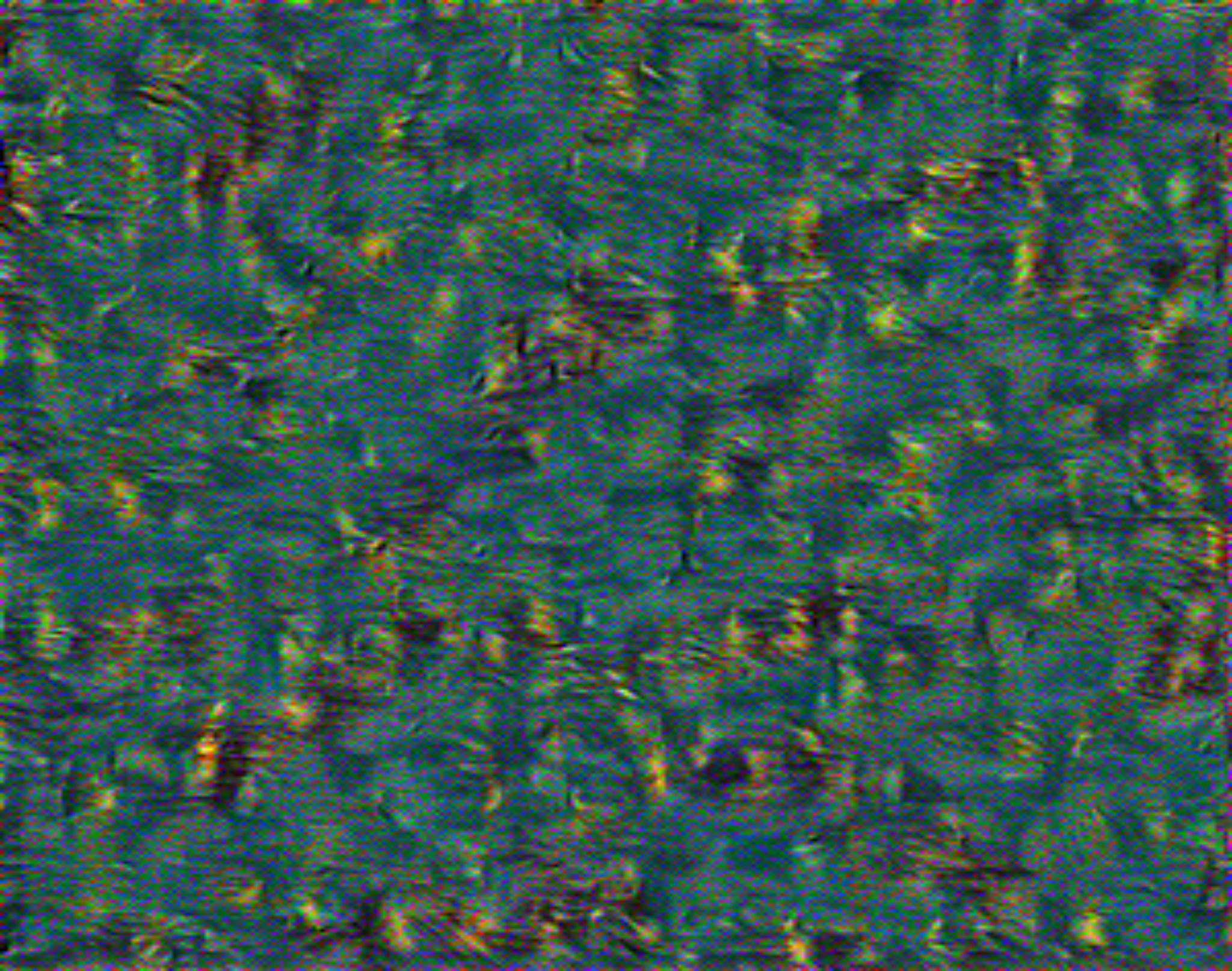
Style Reconstruction

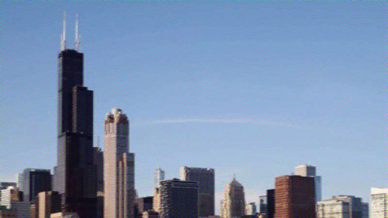
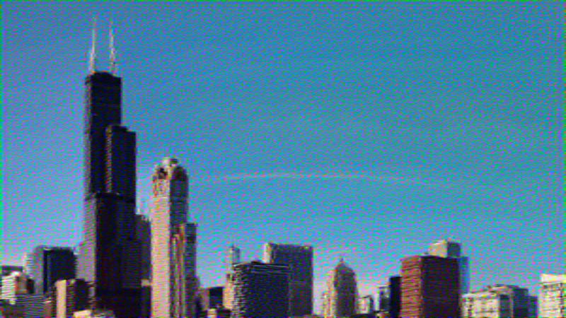
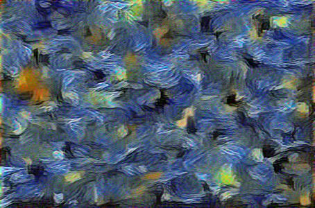
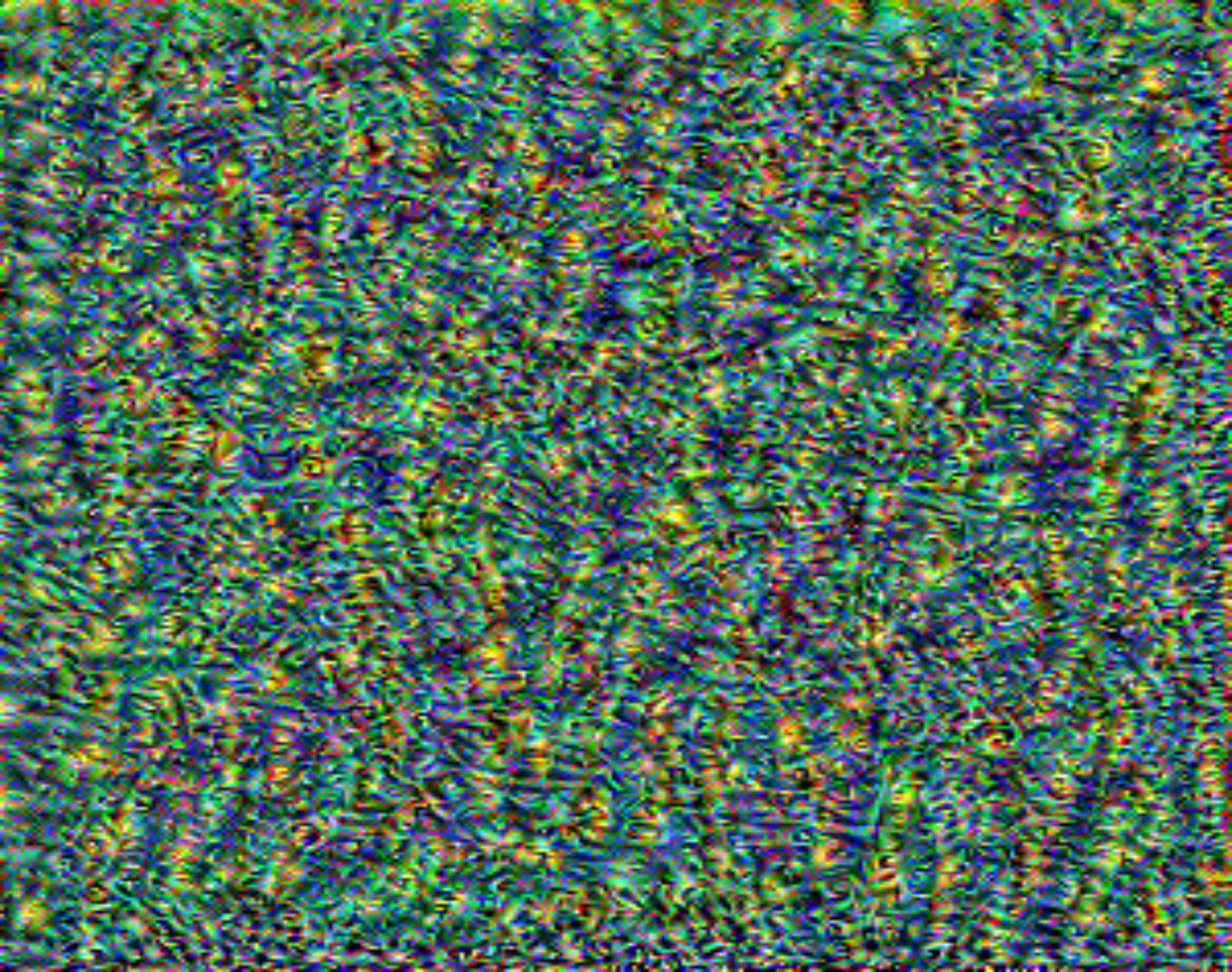
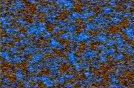
Similarly we run style reconstruction. This time we set $\alpha$ to 0 and we only use one layer for style loss. Original Images: Reconstructed Style: Stylistically what is interesting is that the first layer is probably the worst at guessing the style of the image. I think this is because there is not enough time for the model to nail the style when each pixel is limited to three channels. It is important for the net to be as expressive as possible and that is only true for the later layers. It seems like the real perceptual style only comes out in layers 6-8. So we will be using that in our style transfer construction.

Style Transfer Results

Now that we have done our reconstruction, we can get a good idea of what layers we want for the content and style layers. For the content layers, we use the 5th convolutional layer. This helps preserve enough structure in the image without being too overpowering of the style loss. For the style loss, we take an average over the 7th, 8th, and 9th convolutional layers to get the most realistic style.

Results

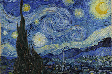
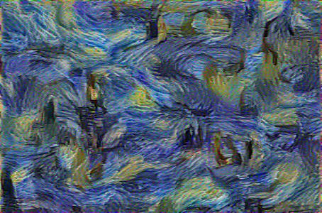
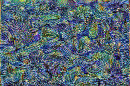
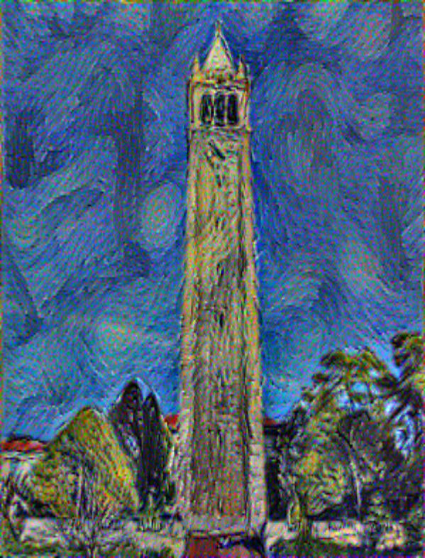
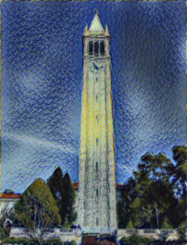
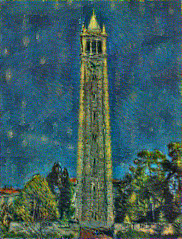
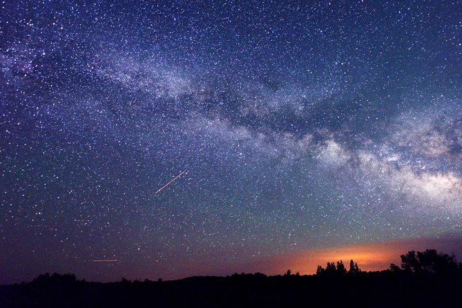
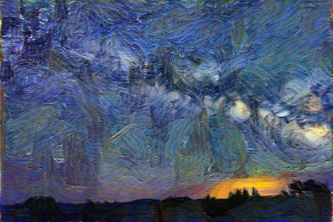
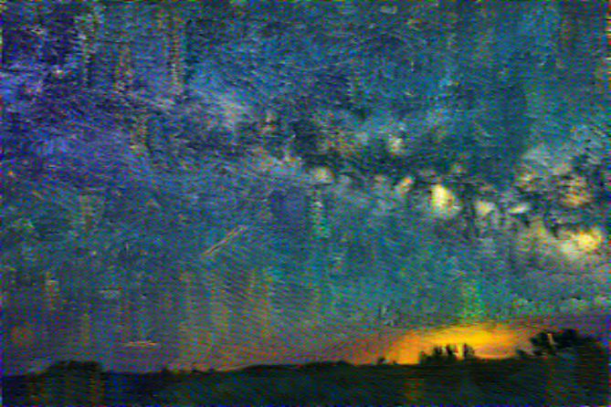
Starry Campanile
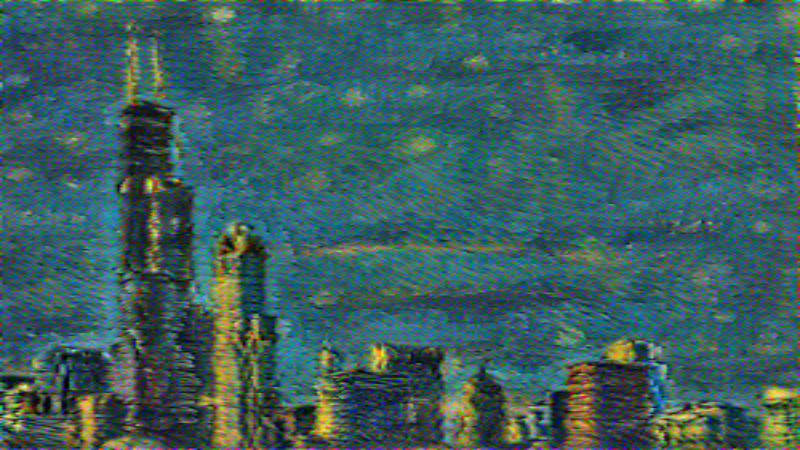
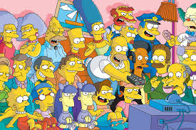
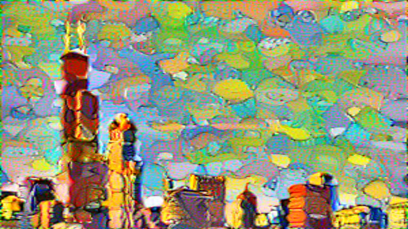
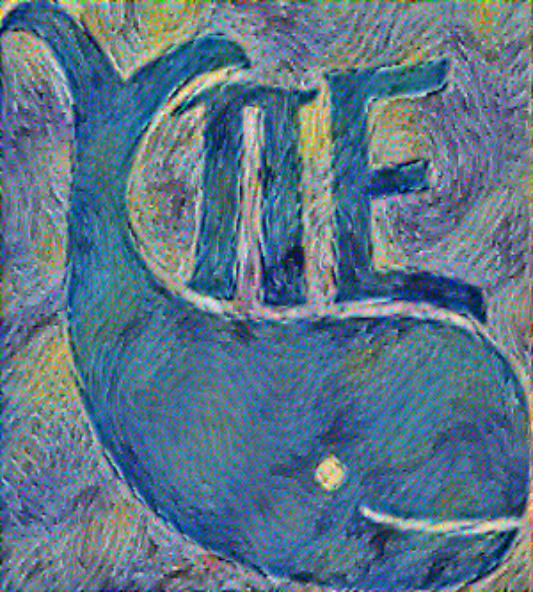
The first one used starry night and the campanile and later layers of the network. The second one used earlier layers of the network. Wild Campanile Wild Chicago Simpsons Chicago Starry Arizona Apocalypse Arizona Whales As a part of my student org, I also made whales in different styles