Bells & Whistles
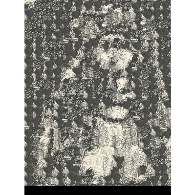
We can make result better using image quilting together with blending (e.g. feathering or Laplacian pyramid). In this example of using toast texture to produce a face, we can blend the output face together with original toast sample using Laplacian pyramid to produce a smooth face-in-toast image.

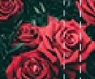
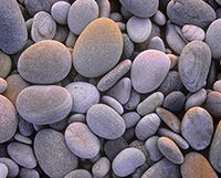
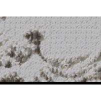
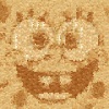
Sample: toast
67 * 63

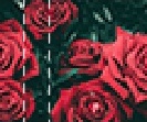
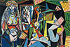
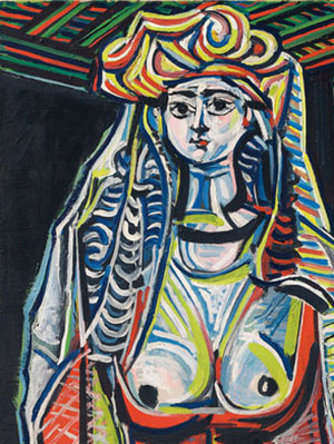
Target image
100 * 100
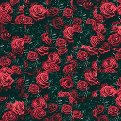
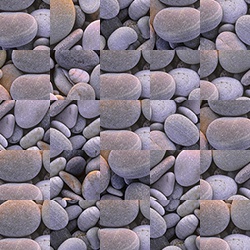
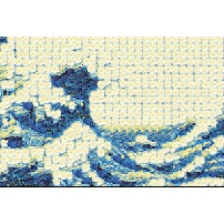
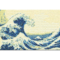
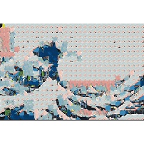
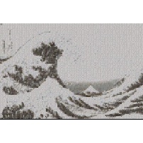
Texture transfer result
patch size: 5
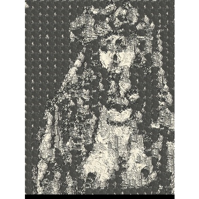
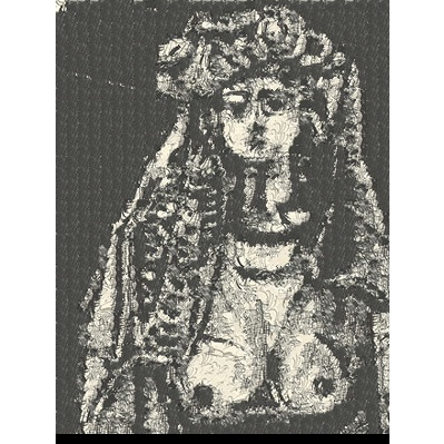
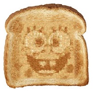
To put the result back on to the toast, I resized the toast to 200 * 183 and texture transfer result to a size fit into the toast. Below are results of puting the texture transfer reault directly on the toast (left )and using Laplacian pyramid with 2 layers to blend them together (right).
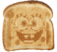
Puting the texture transfer reault directly on the toast.
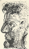
Blended using Laplacian pyramid.
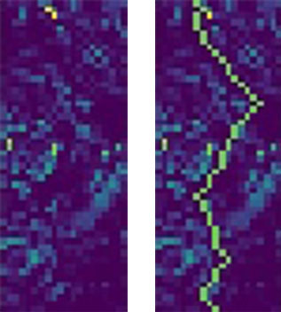
Below are Laplacian pyramid elements. Result is computated by:
im1_layer1 = Laplacian_filter(image1, sigma=1)
im2_layer1 = Laplacian_filter(image2, sigma=1)
filter_layer1 = Gaussian_filter(image3, sigma = 1)
im1_layer2 = im1 - im1_layer1
im2_layer2 = im2 - im2_layer1
filter_layer2 = Gaussian_filter(image3, sigma = 2)
result = im1_layer1*filter_layer1 + im2_layer1*(1-filter_layer1)
+ im1_layer2*filter_layer2 + im2_layer2*(1-filter_layer2)
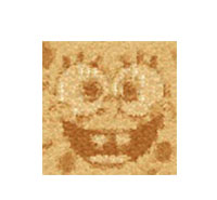
Image1: Image to blend in.
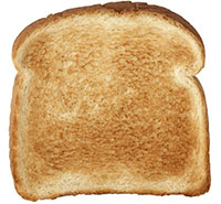
Image 2: Background image.
Image 3: Filter.