Final Project: Lightfield Camera and Gradient Domain Fusion
Project Overview
For my final project, I decided to tackle the Lightfiend Camera and
Gradient Domain Fusion tasks, both which provided their own sets of unique
challenges. Join me in exploring the beauty of image manipulation one final time :)
Final Project Link
Lightfield Camera
A lightfield camera (also known as a plenoptic camera) captures images by absorbing light rays from every possible direction, allowing one to generate photos in 3D
space that look like "living pictures". This project explores how lightfield data can be manipulated with simple operations (i.e. shifting and averaging) to produce different effects on the overall
image. The lightfield data was taken from Stanford's Light Field Archive.
Part 1: Depth Refocusing
When generating lightfield data, we move the camera and have it capture photos from a variety of angles. If we move the camera while keeping the lens' optical axis unchanged,
objects that are closer to the camera vary their positions significantly between images whereas objects that are farther don't vary as much. Therefore, averaging all the lightfield
images together without modifications generates a photo with nearby objects appearing blurry and far-away objects appearing sharp. We can take advantage of this phenomenon to
generate images that focus on different objects at different depths (i.e. depth refocusing).
Each lightfield dataset contains 289 sub-aperture images Ix, y in a 17x17 grid (0-indexed) with corresponding (u, v) values to signify the camera's location.
We define the center image as I8, 8 with a corresponding (uc, vc) location. To refocus an image, we first shift every image Ix, y
in the lightfield by C * (uI - uc, vI - vc) (i.e. shift every sub-apeture towards the center image), then average all the images together. This intuitively "refocuses"
the camera towards a center point. Different values of C will cause the camera's focus to change locations.
Some examples of this are provided below for different C values.
Chess Depth Refocus (C=-0.15 to C=0.65)
Knight Depth Refocus (C=-0.55 to C=0.45)
Part 2: Aperture Adjustment
Additionally, we can simulate readjusting the aperture by averaging only a subset of images within our lightfield datasets. Specifically, the more images we average together, the larger our aperture is, and the larger the aperture is, the more "focused-in" the camera is at a specific point. We determine which images to average using a radius parameter r, where r represents the maximum distance a sub-aperture can be from the center image (according to their (u, v) positions). A couple examples are listed below showing the transition from using one image to all images (289).
Chess Aperture Adjustment (C=0.2, r=0 to r=60)
Knight Aperture Adjustment (C=-0.175, r=0 to r=100)
Summary
Overall, I thought it was interesting how sub-apertures within lightfield data could be combined in very simple ways to simulate changes in depth and aperture, simulating effects that are now commonplace in modern cameras and smartphones. It also gave me a new perspective in image processing, as it helps bridge the gap between the 3D world (represented by light values and directions) and the 2D world (pixels on a flat screen) in a fun and interesting way.
Gradient Domain Fusion
In Project 2, I explored different ways of blending images together
using Gaussian and Laplacian stacks. Although this method worked well, it was frustrating having to create masks that fit each image perfectly (i.e. perfect
cut-outs of the source image to blend into the target image). To remedy this issue, we explore the concept of Poisson Blending. Poisson Blending works by setting up a systems of equations that maximally preserves the gradients of the source image while keeping all the background pixels
the same. This fundamentally ignores the intensity of our pixel values (i.e. emphasis on image features over color) but is still quite effective.
Part 1: Toy Problem
Before implementing Poisson Blending, let's attempt to reconstruct a toy image S of dimension (h, w) using only x and y gradients.
To do this, we want to solve the systems of equations Av = b, where v is a vector with length h * w that represents a flattened image
equivalent to the source image S
We set-up our systems of equations with the following:
- Flatten the 2D image S into a 1D vector s with length h * w
- Create a matrix A with dimensions (2 * h * w + 1, h * w). This matrix acts as the gradient operator
- The first h * w rows represent the x-gradients of S (where s(x+1, y) - s(x, y) = v(x+1, y) - v(x, y))
- The next h * w rows represent the y-gradients of S (where s(x, y+1) - s(x, y) = v(x, y+1) - v(x, y))
- The last row represents the constraint s(0, 0) = v(0, 0). This is necessary for generating a unique solution for v (without this condition, we could generate an infinite amount of solutions by adding an arbitrary constant value to v)
- Generate vector b with length h * w by setting it to A @ s. This vector represents the gradients of s
Solving Av = b generates a near-replica of the original flattened image s. The before and after are shown below with a MSE error of 7.678e-12.
- NOTE: these images are not the same, but they look nearly identical.
Toy Image (S)

Generated Image (V)
Part 2: Poisson Blending
Now that we've solved the toy problem, we can implement Poisson Blending! Poisson Blending attempts to minimize the following equation:

Let v be the resulting image, s is the flattened source image that we want to blend, and t is the flattened target image that we are
blending s into. Additionally, S in this case refers to the set of pixels that are contained within our defined mask (i.e. the pixels that we
want to blend into the target image). Ni refers to the 4-neighbors of i (i.e. the pixels directly above/below and left/right of i).
The first equation attempts to minimize the gradients between our source image inside the mask and the resulting image v. The second equation captures the
edge case where one of the neighbors fall outside of the mask: in that case, we use the target image t as the parameter for that specific gradient.
We can set-up the above minimization problem as a system of equations Av = b:
- Let A be a matrix with dimensions (h * w, h * w) and b be a vector of length h * w (1 row for each pixel in s)
- For each numbered pixel i in s:
- If the current pixel is outside the mask S, set-up the equation: s(x, y) = t(x, y) in row Ai, bi
- If the current pixel is inside the mask S, for each neighbor n of si:
- Add the equation: s(x, y) - n(x, y) to Ai
- Add the equation: t(x, y) - n'(x, y) for t's corresponding neighbor to bi
- Note: If the neighbor n falls outside of the mask, replace n(x, y) in A with n'(x,y)
A few examples of this are shown below:
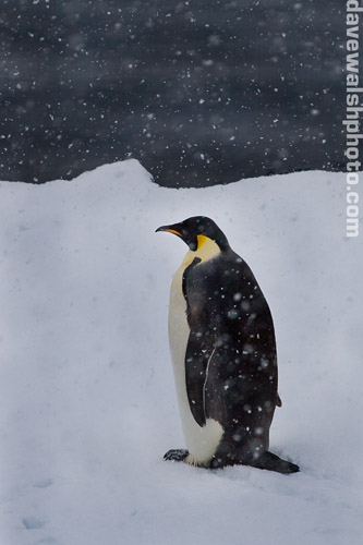
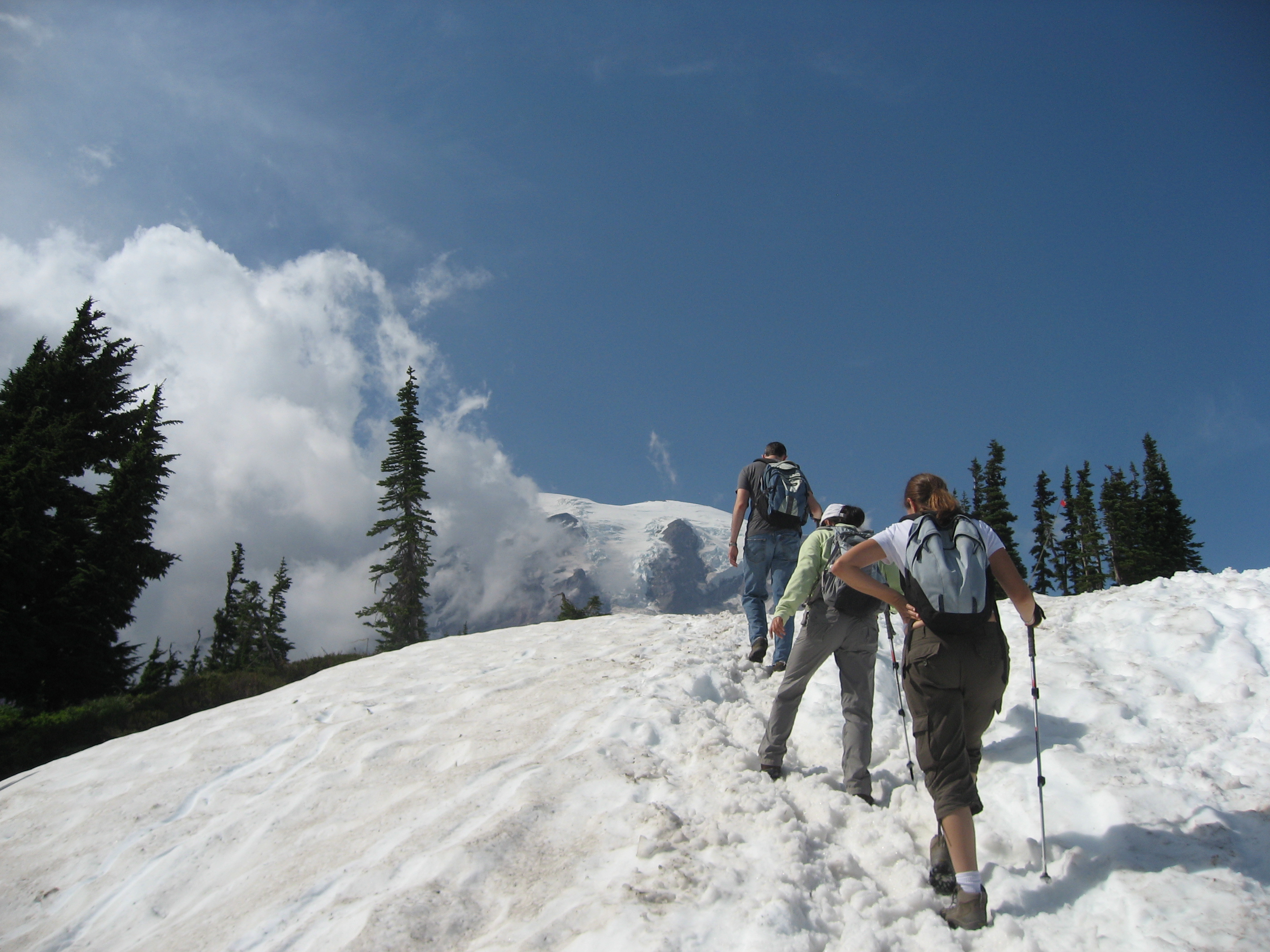
Penguin (Source)
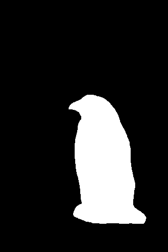
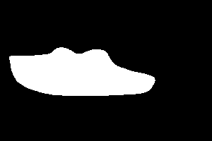
Penguin (Mask)
Snowy Hill (Target)
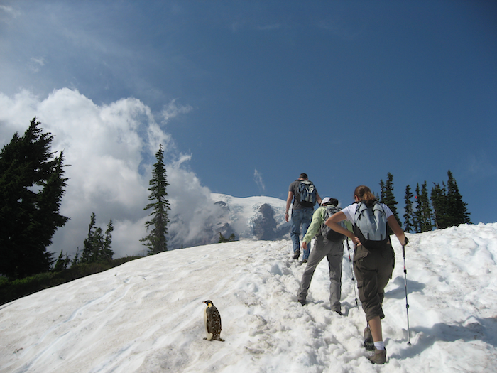
Naive Penguin Blend

Poisson Penguin Blend
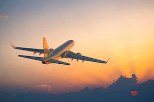
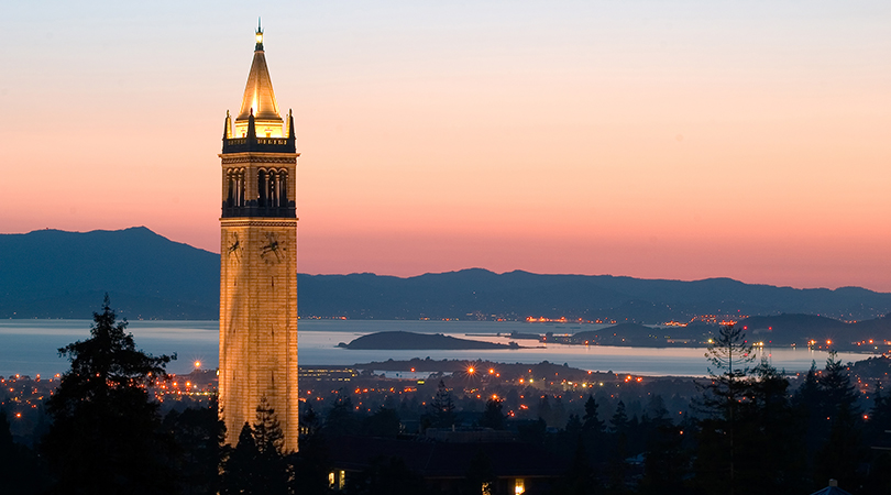
Plane (Source)
Plane (Mask)
UCB Sunset (Target)
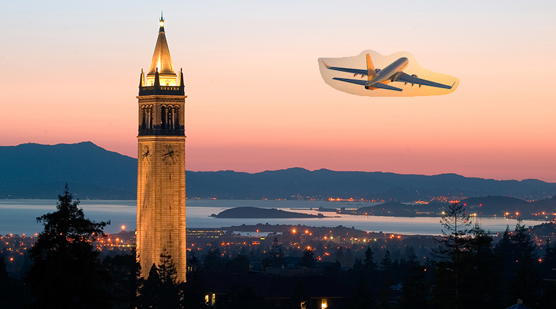
Naive Sunset Blend
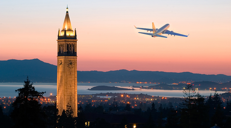
Poisson Sunset Blend
Moon (Source)
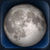
Moon (Mask)
Aurora (Target)
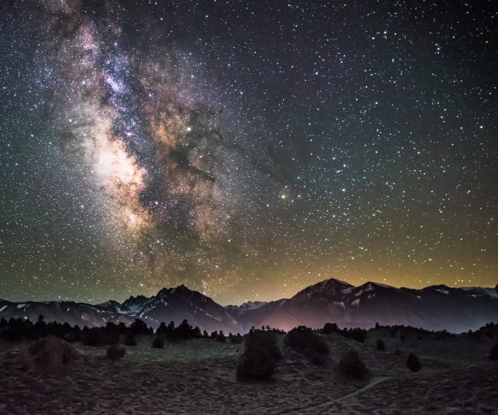
Naive Night Blend
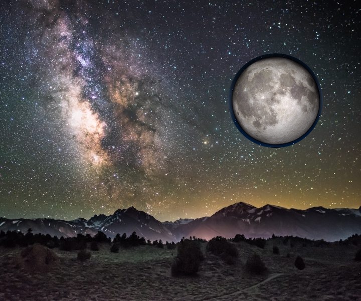
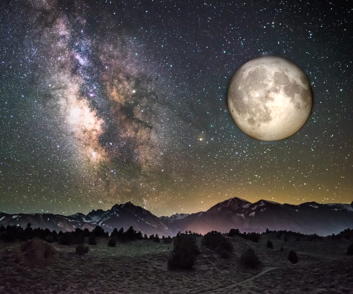
Poisson Night Blend
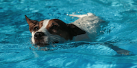
Doggo (Source)
Doggo (Mask)
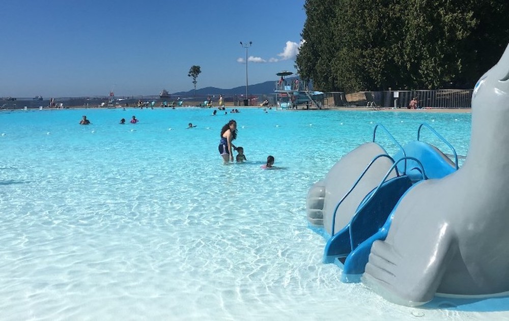
Pool (Target)
Naive Pool Blend
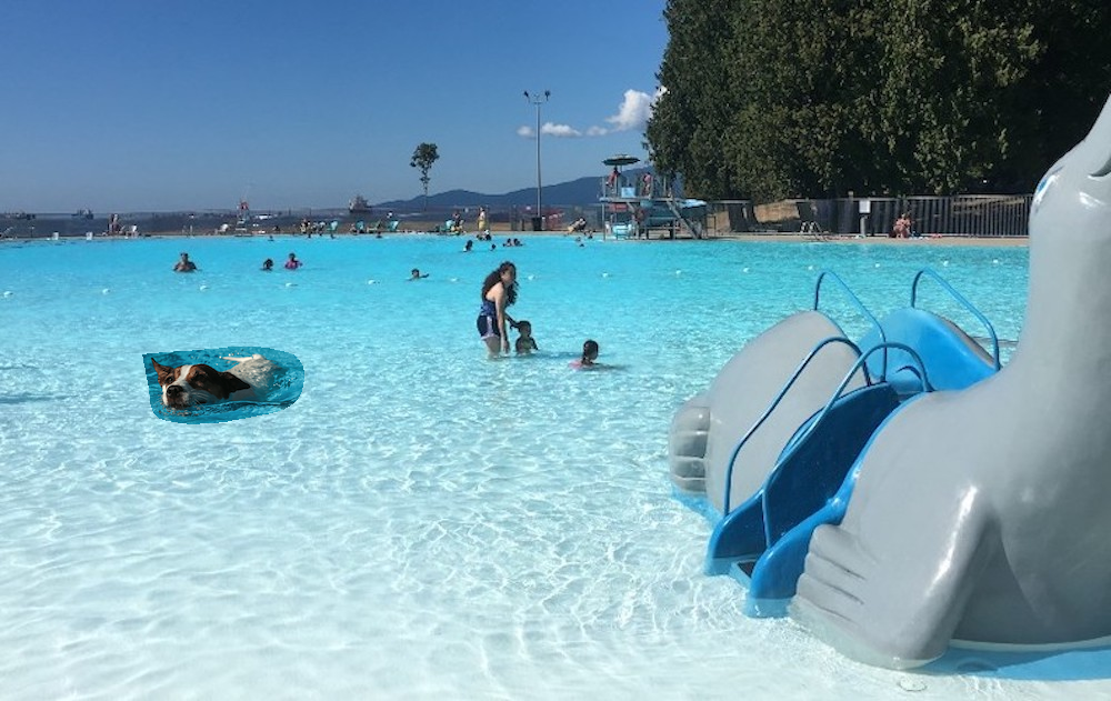
Poisson Pool Blend
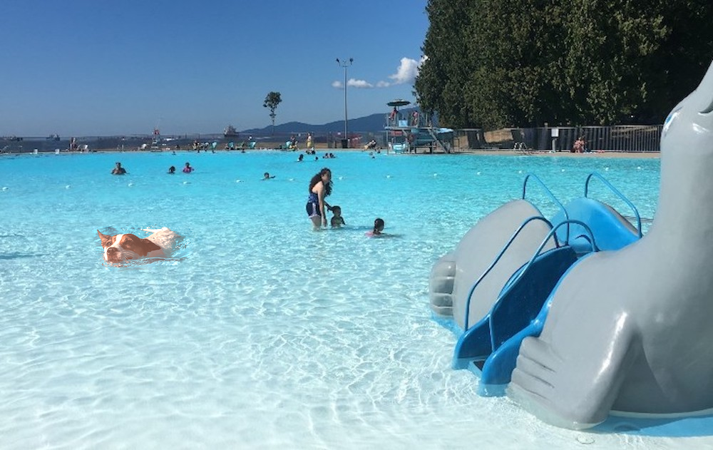
The blends that performed the best were sources whose background colors matched those of their targets (in this case, the Penguin and Sunset examples). However, this blending technique isn't perfect. In the pool example, since the source image's pool water was drastically darker than the target image, the blend (although maintaining details well) significantly altered the coloring of the original dog in an attempt to preserve the images' gradients. Additionally, the moon example, although more effective than the naive approach, has a slight blurred border since the source image's background (all black) doesn't line up nicely with the target image (aurora stars).
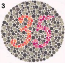
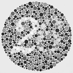
Bells and Whistles: Color2Gray
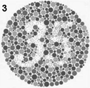
Although I did not complete the mixed gradients bells and whistles, I attempted to solve the Color2Gray problem, where sometimes converting a color image to grayscale
would result in the loss of contrast information. We explore this phenomenon in the context of colorblind number tests. Instead of doing the naive approach (convert
to grayscale with only rgb2gray), we first take the source image S and convert it into its HSV format (Hue-Saturation-Value) H.
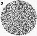
To convert the image into grayscale:
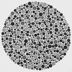
- Generate the naive grayscale image N by using rgb2gray
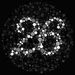
- Create a binary mask from the saturation values of H (i.e. greater than 0.2 threshold)
- Copy the "value" values of H into N based on the mask to generate the final output
35 (Colorized)
35 (Rgb2Gray)
35 (Saturation Mask)
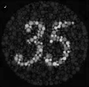
35 (Color2Gray)
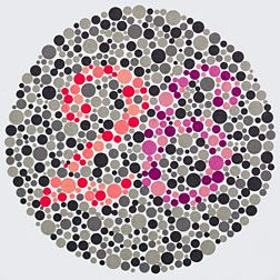
26 (Colorized)
26 (Rgb2Gray)
26 (Saturation Mask)
26 (Color2Gray)
Summary
In the end, it was nice to explore another method of blending that did not rely on creating the perfect mask. In the above examples,
the masks were cropped fairly sloppily (i.e. leaving behind some background information was fine since those errors were smoothed out
across the gradient calculation). I also found it fascinating that Poisson blending was vested heavily within mathematics (calculating
gradients) whereas the previous project (Multiresolution blending) involved using Gaussian filters to achieve a similar goal. Overall,
this was a very fun project to work on.
That's the end of my CS 194-26 journey! Thanks for a great semester :)