Gradient of a function
The gradient of a differentiable function  contains the first derivatives of the function with respect to each variable. As seen here, the gradient is useful to find the linear approximation of the function near a point.
Definition
Composition rule
Examples
Geometric interpretation
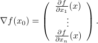
Definition
The gradient of  at
at  , denoted
  , is the vector in
  given by
Examples:
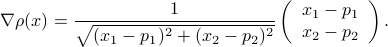
Distance function: The distance function from a point
 to another point
  is defined as

The function is differentiable, provided  , which we assume. Then
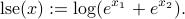
Log-sum-exp function: Consider the ‘‘log-sum-exp’’ function
 , with values
The gradient of  at
at  is
is
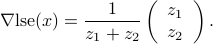
where  ,
,  . More generally, the gradient of the function
  with values
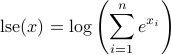
is given by

where 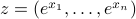 , and
, and  .
.
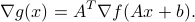
Composition rule with an affine function
If  is a matrix, and
  is a vector, the function
  with values
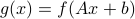
is called the composition of the affine map  with . Its gradient is given by (see here for a proof)
Geometric interpretation
Geometrically, the gradient can be read on the plot of the level set of the function. Specifically, at any point , the gradient is perpendicular to the level set, and points outwards from the sub-level set (that is, it points towards higher values of the function).
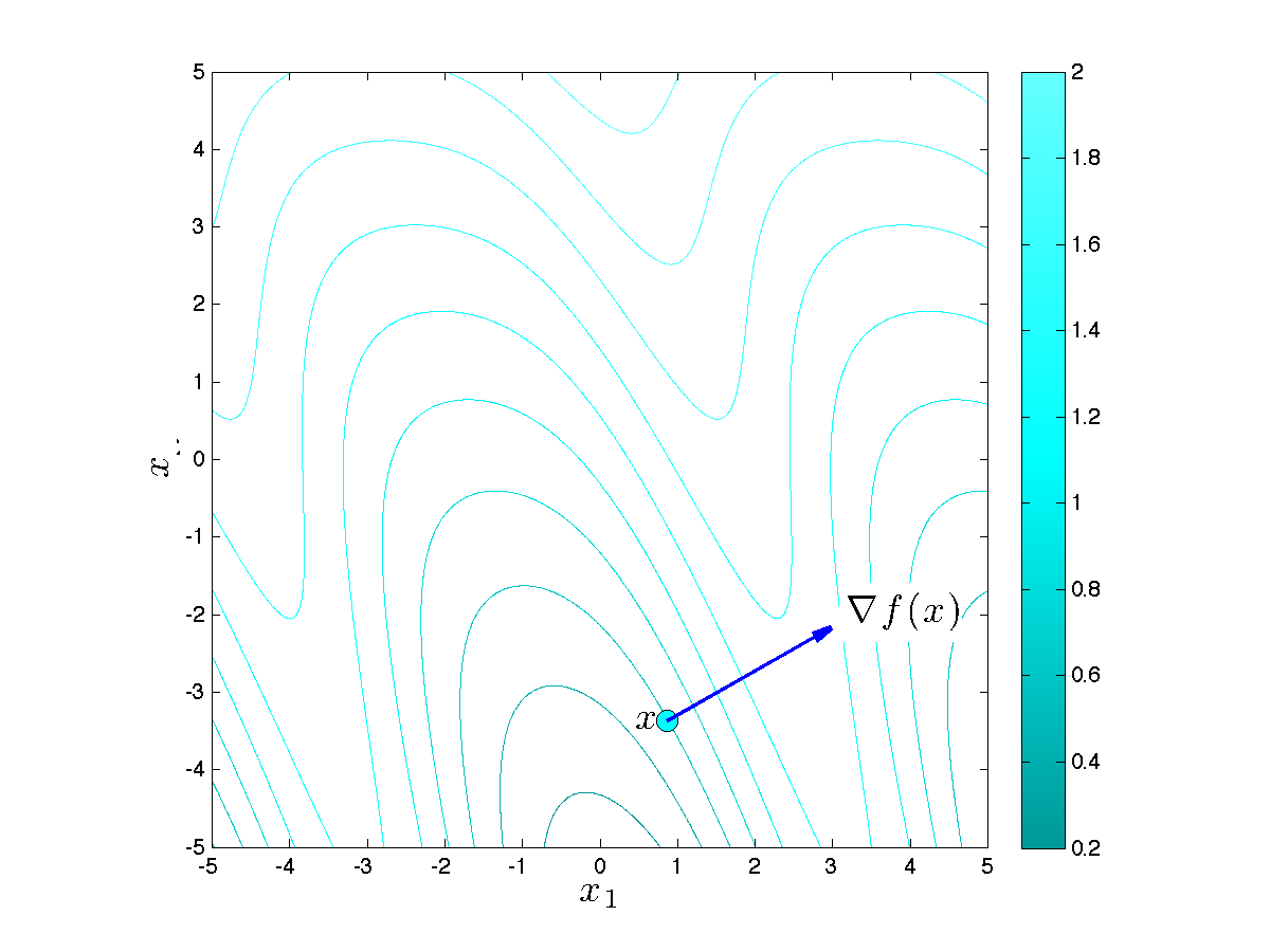 |
Level and sub-level sets of the function 
The gradient at a point (shown in red) is perpendicular to the level set, and points outside the corresponding sub-level set. The length of the gradient determines how fast the function changes locally (The length of the gradient has been scaled up by a factor of |
 .)
.)