Implementation Errors in an Antenna Array Design Problem

Return to the antenna array design problem described here. Let us specifically consider the problem of minimizing the sidelobe level subject to a normalization constraint, described here. This problem takes the form of an SOCP:

$min_{z in mathbf{C}^n, : delta} : delta ~:~ mbox{bf Re}(D_z(0)) ge 1, ;; |D_z(phi_i)| le delta, ;; i=1,ldots,m.$

Uncertainty model

We assume that the antenna weights (contained in the complex vector $z^ast in mathbf{C}^n$ ) are subject to implementation errors. It is natural to model these errors as multiplicative perturbations on the antenna weights, of the form

where the relative errors $xi_k in mathbf{C}$ are bounded: |xi_k| le rho , k=1,ldots,n . Here, rho is a measure of the maximum amount of implementation errors.

Note that such uncertainty errors amount to uncertainties in the coefficients of the original SOCP.

Impact on solution

Assume that we have solved the above SOCP, and found a solution z^ast .

Now let us perturb the solution according to the uncertainty model above. We generate random samples of the relative error vector $xi in mathbf{C}^n$ , inside the box ${ xi ::: |xi|_infty le rho}$ .

When we change the antenna weights, the normalization requirement $mbox{Re}(D_z(0)) ge 1$ is not necessarily met. To compare diagrams meaningfully, we scale the sample diagrams to make |D(0)| equal to , and look at the resulting diagrams.

When solving the problem with nominal data and an equidistant -point angular grid, we end up with the nice nominal solution depicted here. For this solution and no data perturbations, the optimal sidelobe level is as low as delta^ast = 0.0048 .

Unfortunately, these nice results are nothing but a dream. In reality, with random actuation errors of level as low as rho = 0.01 % , our supposedly optimal design becomes a complete disaster. With 1000 samples, the sidelobe level for the nominal design jumps, on the average, from its nominal value 0.0048 to 1.2342 , even attaining a maximum of 29.7889 ! In fact, in some of these random realizations of the diagram, most of the energy is sent in the opposite direction, as seen below.

The dream: the optimal magnitude diagram. The attenuation is excellent in the stop band, so that the stop-band magnitude is not distinguishable from zero in this plot.

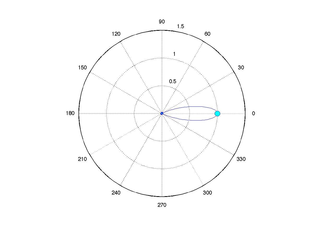
The reality: a particular magnitude diagram obtained after perturbing the optimal weights of the above design with a relative error of 0.01% . This design is a complete disaster: most of the energy is sent in the opposite direction from the target.

The reality: another particular magnitude diagram obtained after perturbing the optimal weights of the above design with a relative error of 0.01% . This design is also a complete disaster: the sidelobe level is has jumped from 0.0048 to almost , an increase by four orders of magnitude.

What is going on?

What happens is that the optimal antenna weights are quite high in magnitude, to the order 10^3 - 10^4 . Thus, even a small relative error in the weights can have consequences. The physics of our setup does not help: the distances between consecutive oscillators is equal to 1/8 of the wavelength, and the spatial angle of interest — the one where we would like to send as much energy as possible — is comprised of directions whose angular distances from the axial direction are at most 30^o .

This is a problem similar to what happens when trying to find a solution to a least-squares problem where the data matrix has low rank: the solution is highly sensitive to changes in the data.