Piece-wise constant fitting

We observe a noisy time-series (encoded in a finite-dimensional vector ) which is almost piece-wise constant. The goal in piece-wise constant fitting is to find what the constant levels are. In biological or medical applications, such levels might have interpretations as ‘‘states’’ of the system measured.

Unfortunately, the signal is not exactly piece-wise constant, but a noisy version of such a signal. Thus, we seek to obtain an estimate of the signal, say hat{x} , such that hat{x} has as few changes in it as possible. We model the latter by minimizing the cardinality of the ‘‘difference’’ vector , where is the difference matrix

D = left[ begin{array}{ccccc}-1 & 1 & 0 & ldots & 0 0 &-1 & 1 & ldots & 0 &&& ddots & ldots & & 0 &-1 & 1 end{array} right].

Matrix is constructed so that $Dx =(x_2-x_1,x_3-x_2,ldots,x_n-x_{n-1})$ .

We are led to the problem

$min_{hat{x}} : |x - hat{x}|_2^2 ~:~ mbox{bf Card} (Dx) le K,$

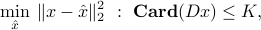
where is an estimate on the number of jumps in the signal. Here, objective function in the problem is a measure of the error between the noisy measurement and the estimate hat{x} .

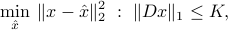
The l_1 -norm heuristic consists in replacing the top (hard) problem by the QP:

$min_{hat{x}} : |x - hat{x}|_2^2 ~:~ |Dx|_1 le K,$

CVX implementation
cvx_begin
    variable x(n)
    minimize( sum_square(y-x) )
    subject to
       norm(D*x,1) <= K;
cvx_end

Piece-wise constant fitting. Top panel: the true signal and its noisy version. Middle: l_1 -constrained fitting, showing a good fit with the true (unknown) signal. Bottom: l_2 -constrained fitting.