Dual Problem
Primal problem
Lagrange function
Dual function
Dual problem
Remarks
Primal Problem
We consider a constrained optimization problem in standard form:

We will refer to this problem as the primal problem. Its optimal value is the primal value, and  denotes the primal variables. We define
  to be the constraint map, with values
  .
.
Example: the problem of finding the minimum distance to a polyhedron can be written as
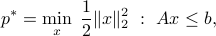
for appropriate matrix  and vector
  .
.
Lagrange function
We define the Lagrange function to be a function  with values
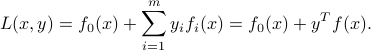
The Lagrange function depends on on the primal variables and an additional variable  , referred to as the dual variable.
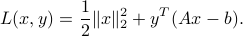
Example: The problem of minimum distance to a polyhedron above admits the Lagrangian
Dual function
Based on the Lagrangian, we can build now a new function (of the dual variables only) that will provide a lower bound on the objective value.
For fixed  , we can interpret the partial function
  as a penalized objective, where violations of the constraints of the primal problem incur a penalty. The penalty grows linearly with the amount of constraint violation, and becomes positive only when one of the constraints is violated. Of course, if no constraint is violated, that is, if
  is feasible, then
  . Hence

Define the dual function  with values
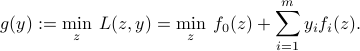
Note that, since  is defined as a point-wise minimum, it is a concave function.
We have, for any  ,
, 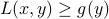 . Putting this together with the previous inequality, we get

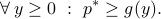
That is, the dual function provides a lower bound on the objective value in the feasible set. The right-hand side of the above inequality is independent of . Taking the minimum over in the above, we obtain
Note that our lower bound may or may not be easy to compute. However, at first glance, computing  with
with  fixed seems to be easier than the original problem, since there are no constraints.
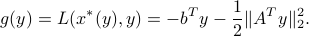
Example: For the problem of minimum distance to a polyhedron above, the dual function is

In this case, the dual function can be computed explicitly. Indeed, the above problem is unconstrained, with a convex objective function (of ), hence global optima are characterized by setting the derivative with respect to to zero. In this case, we obtain a unique optimal point 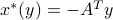 . Replacing by its optimal value, we obtain
Dual problem
Since the lower bound is valid for every , we can search for the best one, that is, the largest lower bound:
The problem of finding the best lower bound:
is called the dual problem associated with the Lagrangian defined above. It optimal value  is the dual optimal value. As noted above, is concave. This means that the dual problem, which involves the maximization of with sign constraints on the variables, is a convex optimization problem.
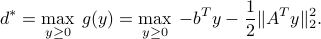
Example: For the problem of minimum distance to a polyhedron above, the dual problem is
Problems with equality constraints
Equality constraints can be simply treated as two inequality ones. It turns out that this ends up being the same as if we simply remove sign constraints in the corresponding multiplier.
Remarks
Via duality, we can compute a lower bound on the optimal value of any problem, convex or not, using convex optimization. Several remarks attenuate the practical scope of the result:
The dual function
may not be easy to compute: it is itself defined as an optimization problem! Duality works best when can be computed in closed form.Even if it is possible to compute
, it might not be easy to maximize: convex problems are not always easy to solve.A lower bound might not be of great practical interest: often we need a sub-optimal solution. Duality does not seem at first to offer a way to compute such a primal point.
Despite these shortcomings, duality is an extremely powerful tool.
Examples:
Bounds on Boolean quadratic programming via Lagrange relaxation.