Alternate maximization

Expectation-Maximization algorithms for Non-Convex Problems

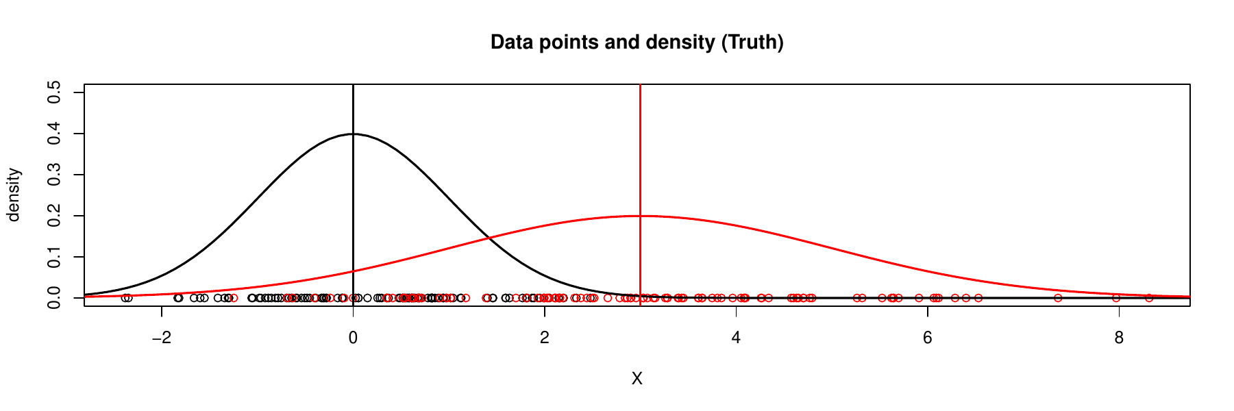
Gaussian mixture statistical models (GMM) is a generalization of the Gaussian model. In a Gaussian 2-mixture model \(X\), we have some chance \(\lambda\) that \(X\sim N(\mu_{1},\sigma_{1}^{2})\) and some chance \((1-\lambda)\) that \(X\sim N(\mu_{2},\sigma_{2}^{2})\). To identify from which component \(X\) comes, we use a label \(Z\) to indicate the component \(X\) belongs to. Hence, we have a prior for \(Z\) as probability that \(X\) is drawn from component 1 or 2:

\[ \boldsymbol{P}(Z=1)=\boldsymbol{P}(Z=1\mid X,\boldsymbol{\theta}) =\lambda, \\ \boldsymbol{P}(Z=2)=\boldsymbol{P}(Z=2\mid X,\boldsymbol{\theta}) =1-\lambda. \]

Let us assume \(\lambda\in(0,1)\) is a known constant for simplicity, say \(\lambda=\frac{1}{2}\). We can also treat this as an unknown parameter to be estimated. In above we assume that the Gaussian mixture statistical model is determined by unknown parameters \(\boldsymbol{\theta}=(\mu_{1},\mu_{2},\sigma_{1}^{2},\sigma_{2}^{2})\). Suppose we can observe the label \(Z\), then a typical dataset would look like

\[ (x_{1},z_{1}) =(0.26,1) \\ (x_{2},z_{2}) =(0.75,1) \\ (x_{3},z_{3}) =(0.23,2) \\ (x_{4},z_{4}) =(0.11,2) \]

We have \(X\mid Z\sim N(\mu_{1},\sigma_{1}^{2})\cdot\boldsymbol{1}(Z=1)+N(\mu_{2},\sigma_{2}^{2})\cdot\boldsymbol{1}(Z=2)\).

\[ \boldsymbol{P}(X=x\mid Z=1,\boldsymbol{\theta}) =\frac{1}{\sqrt{2\pi\sigma_{1}^{2}}}\exp\left(-\frac{(x-\mu_{1})^{2}}{2\sigma_{1}^{2}}\right),\\ \boldsymbol{P}(X=x\mid Z=2,\boldsymbol{\theta}) =\frac{1}{\sqrt{2\pi\sigma_{2}^{2}}}\exp\left(-\frac{(x-\mu_{2})^{2}}{2\sigma_{2}^{2}}\right). \]

For instance, \((X,Z)=(x_{4},z_{4})=(0.11,2)\) means that the observed data \(x_{4}\) comes from component 2, which is indicated by the unobserved values \(z_{4}=2\). This Gaussian mixture component is defined only by \((\mu_{2},\sigma_{2}^{2})\).

The optimization problem we are faced with here is how to estimate the parameter \(\boldsymbol{\theta}\), that is, both \((\mu_{1},\sigma_{1}^{2})\) and \((\mu_{2},\sigma_{2}^{2})\). If we can observe all those \(Z\), then we can simple use \(\{(x_{1},z_{1}=1),(x_{2},z_{2}=1)\}\) for estimating \((\mu_{1},\sigma_{1}^{2})\) and \(\{(x_{3},z_{3}=2),(x_{4},z_{4}=2)\}\) for estimating \((\mu_{2},\sigma_{2}^{2})\) using the maximum likelihood approach as we have seen.

Usually we do not observe \(Z\), and call it an unobserved latent variable. When we cannot observe \(Z\), it is impossible to take the derivatives of likelihood function any more. We can try all possible values of \(Z\) (\(2^{4}\) possibilities in this case), use a Newton-type numerical method (optimizing \(X,Z,\theta\) jointly), but these usually do not work well.

The idea of expectation maximization (EM) algorithm is that we can arbitrarily assign random values to unobserved variables \(Z\) and use these ‘‘guesses’’ to estimate the parameters \((\mu_{2},\sigma_{2}^{2})\), then use estimated values \((\mu_{2},\sigma_{2}^{2})\) to find a better estimate of \((\mu_{1},\sigma_{1}^{2})\), and then keep alternating between the two sets of partial parameters \((\mu_{1},\sigma_{1}^{2})\), \((\mu_{2},\sigma_{2}^{2})\), until the estimated values for the whole \(\boldsymbol{\theta}\) converge. In a sense, this is like a coordinate-wise (or iterative between \(Z\) and \(\boldsymbol{\theta}\)) optimization, or alternate maximization.

• Expectation step (E step): Let \({\displaystyle Q(\boldsymbol{\theta}\mid\boldsymbol{\theta}^{(t)})}\) be the expected value of the log likelihood function of \({\displaystyle \boldsymbol{\theta}}\), with respect to the current conditional distribution of \(Z\) given \(X\) and the current estimates \({\displaystyle \boldsymbol{\theta}^{(t)}}\) of the parameters:

\[ {\displaystyle Q(\boldsymbol{\theta}\mid\boldsymbol{\theta}^{(t)})} \\ =\boldsymbol{E}_{Z\mid X,\boldsymbol{\theta}^{(t)}}\log L(\boldsymbol{\theta}^{(t)}\mid X,Z)\nonumber \\ =\boldsymbol{E}_{Z\mid X,\boldsymbol{\theta}^{(t)}}\log\boldsymbol{P}(X,Z\mid\boldsymbol{\theta})\\ =\lambda\cdot\log\left[\frac{1}{\sqrt{2\pi\sigma_{1}^{2}}}\exp\left(-\frac{(X-\mu_{1})^{2}}{2\sigma_{1}^{2}}\right)\right]\nonumber +(1-\lambda)\cdot\log\left[\frac{1}{\sqrt{2\pi\sigma_{2}^{2}}}\left(-\frac{(X-\mu_{2})^{2}}{2\sigma_{2}^{2}}\right)\right]\label{eq:Q} \]

Note that the \(\boldsymbol{E}_{Z\mid X,\boldsymbol{\theta}^{(t)}}\) in the last step would integrate out all \(Z=(z_{1},z_{2})\) in the expression, therefore, we would have \({\displaystyle Q(\boldsymbol{\theta}\mid\boldsymbol{\theta}^{(t)})}\) as a function of \(\boldsymbol{\theta}\) only, if \(\boldsymbol{\theta}^{(t)}\) and \(X\) are given.

• Maximization step (M step): \({\displaystyle \boldsymbol{\theta}^{(t+1)}=\arg\max_{\boldsymbol{\theta}}\ Q(\boldsymbol{\theta}\mid\boldsymbol{\theta}^{(t)})}\). For this simple model, we can compute the components of \(\boldsymbol{\theta}^{(t+1)}\).

A simple justification of EM algorithm is that

\[ \log L(\boldsymbol{\theta}\mid X) \\ =\log\boldsymbol{P}(X\mid\boldsymbol{\theta})\\ =\log\int\boldsymbol{P}(X,Z\mid\boldsymbol{\theta})d\boldsymbol{P}(Z)\\ =\log\int\frac{\boldsymbol{P}(X,Z\mid\boldsymbol{\theta})}{\boldsymbol{P}(Z\mid X,\boldsymbol{\theta}^{(t)})}\boldsymbol{P}(Z\mid X,\boldsymbol{\theta}^{(t)})d\boldsymbol{P}(Z)\\ =\log\boldsymbol{E}_{Z\mid X,\boldsymbol{\theta}^{(t)}}\frac{\boldsymbol{P}(X,Z\mid\boldsymbol{\theta})}{\boldsymbol{P}(Z\mid X,\boldsymbol{\theta}^{(t)})}\\ (\text{Jensen inequality}) \\ \geq\boldsymbol{E}_{Z\mid X,\boldsymbol{\theta}^{(t)}}\log\frac{\boldsymbol{P}(X,Z\mid\boldsymbol{\theta})}{\boldsymbol{P}(Z\mid X,\boldsymbol{\theta}^{(t)})}\\ =\boldsymbol{E}_{Z\mid X,\boldsymbol{\theta}^{(t)}}\log\boldsymbol{P}(X,Z\mid\boldsymbol{\theta})-\boldsymbol{E}_{Z\mid X,\boldsymbol{\theta}^{(t)}}\log\boldsymbol{P}(Z\mid X,\boldsymbol{\theta}^{(t)})\\ =Q(\boldsymbol{\theta}\mid\boldsymbol{\theta}^{(t)})-\boldsymbol{E}_{Z\mid X,\boldsymbol{\theta}^{(t)}}\log\boldsymbol{P}(Z\mid X,\boldsymbol{\theta}^{(t)}) \]

So we can view \(Q(\boldsymbol{\theta}\mid\boldsymbol{\theta}^{(t)})\) as a convex surrogate of the log likelihood \(\log L(\boldsymbol{\theta}\mid X)\), which is non-convex. As an exercise, can you check the non-convexity of this \(\log L(\boldsymbol{\theta}\mid X)\)?

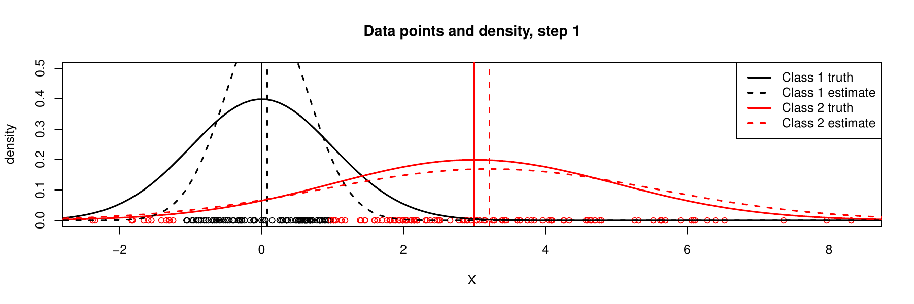
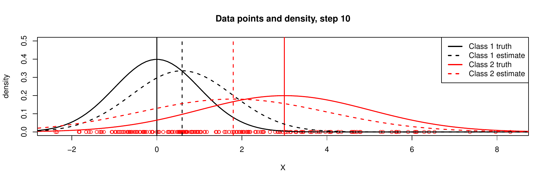
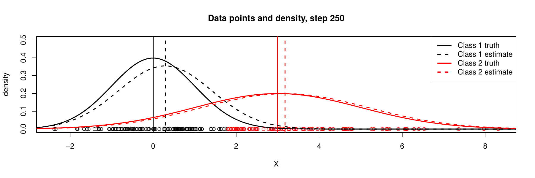
It is always a problem to check whether such an iterative algorithm converge, i.e., whether we finally reach to ideal solution. We would show a sequence of iterations below. By observing that the values of \(\boldsymbol{\theta}\) stabilizes after several iterations and the estimated densities for each component becomes closer to the truth, we would have more confidence in convergence of EM. We do not address this important theoretical problem here in details, but we give following reference paper (known as the ‘‘DLR paper’’):

Dempster, A. P., Laird, N. and Rubin, D. B. (1977), Maximum likelihood from incomplete data via the EM algorithm. https://doi.org/10.1111/j.2517-6161.1977.tb01600.x