Least-Squares Design

Example data

For our particular example, we have the following parameters:

• Number of antennas: .

• Wavelength: .

• Pass-band size: . In what follows, we use the following matlab applet to define the data of our problem.

N = 10; % discretization parameter
n = 16; % number of antennas
lambda = 8; % wavelength
Phi = pi/6; % sidelobe parameter

Least-squares approach

We examine how least-squares can be used to strike a trade-off between the sideloble level attenuation and thermal noise power. The initial problem reads

The basic idea is to penalize the constraints, as follows: we choose a ‘‘trade-off parameter’’ and solve the problem

Remember that the function is linear in :

Hence, the above problem is a linearly constrained least-squares problem.

CVX implementation

The above problem can be solved via linear algebra (SVD) methods. Here, we do not even bother to invoke SVD — CVX will do. A CVX implementation of this problem is given below. Note how we use a new vector variable to handle the objective function. Note also that CVX understands complex variables.

Angles = linspace(Phi,pi,N); % angles in the stop band
a = 2*pi*sqrt(-1)/lambda; % intermediate parameter
cvx_begin
    variable z(n,1) complex;
    variable r(N,1) complex;
    minimize( z'*z+mu*r'*r )
    subject to
        for i = 1:N,
            exp(a*cos(Angles(i))*(1:n))*z == r(i);
        end
        real( exp(a*(1:n))*z) >= 1;
cvx_end

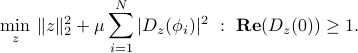
Antenna array design via least-squares: minimal combination of thermal noise and sidelobe level violations, computed at points, with trade-off parameter . The corresponding sidelobe attenuation level is , and the thermal noise power is .

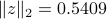Note that the penalty approach adopted here will not enforce the desired constraints. We can only hope that, for large enough, all of the terms in the sum will go below the desired threshold . In practice, we expect that some terms might not. It seems to be hard to achieve the best trade-off this way. The following plot shows the trade-off curve that we can achieve.

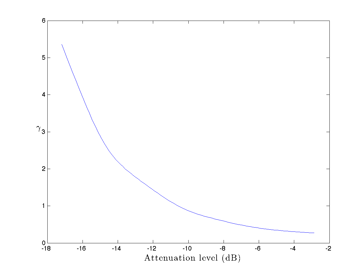Trade-off curve achieved via via least-squares.