Standard Forms of GP

GP > Posynomials | Standard Forms | Applications

Geometric Programs
Convex Form
CVX Syntax

Standard Form

A geometric program (GP for short) is a problem with generalized posynomial objective and inequality constraints, and (possibly) monomial equality constraints.

In standard form, a GP can be written as

min_x : f_0(x) ~:~ f_i(x) le 1, ;; i=1,ldots,m, ;; h_j(x) = 1, ;; j=1,ldots,p,

where f_0,ldots,f_m are generalized posynomials and h_1,ldots,h_p are monomials.

Assuming for simplicity that the generalized posynomials involved are ordinary posynomials, we can express a GP explicitly, in the so-called standard form:

$min_x : sum_{k=1}^{K_0} c_{k0} x^{a_0} ~:~ begin{array}[t]{l} displaystylesum_{k=1}^{K_i} c_{ki} x^{a_{ki}} le 1, ;; i=1,ldots,m, g_j x^{f_j} = 1, ;; j=1,ldots,p. end{array}$

where a_0,ldots,a_m and c_1,ldots,c_m are vectors in $mathbf{R}^n$ , and c_i > 0 , k=1,ldots,m , g > 0 are vectors with positive components. In the above, we follow the power law notation.

Converting the problem into the standard form when the original formulation involves generalized posynomials entails adding new variables and constraints (see here).

Example: Optimization of a water tank.

Convex Form

GPs in standard form are not convex, but a simple transformation allows to put them into an equivalent, convex form. The idea, already seen in the context of posynomial functions, is to take logarithms of the original variables. Again we assume that the posynomials involved are not generalized posynomials, but ordinary ones.

Consider a posynomial constraint of the form

$f(x) := sum_{k=1}^K c_k x^{a_k} le 1 .$

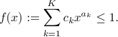
where the vector has positive components: c >0 . We can express this constraints in terms of the new variable $y in mathbf{R}^n$ , defined as y_i = log x_i , i=1,ldots,n :

$log f(x) = mbox{bf lse}(Ay+b) := log left( sum_{k=1}^K e^{a_k^Ty + b_k} right) le 0,$

where b_k := log c_k , k=1,ldots,K , is the K times n matrix with rows a_1,ldots,a_K , and mbox{bf lse} is the log-sum-exp function.

Note that if the posynomial was actually a monomial, there would be only one term in the mbox{bf lse} function, and the constraint would reduce to an ordinary affine inequality.

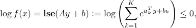
Since the log-sum-exp function is convex, the above constraint is actually convex in the new variable .

By this argument, the GP

$min_x : displaystylesum_{k=1}^{K_0} c_{k0} x^{a_{k0}} ~:~ begin{array}[t]{l} displaystylesum_{k=1}^{K_i} c_{ki} x^{a_{ki}} le 1, ;; i=1,ldots,m, g_j x^{f_j} = 1, ;; j=1,ldots,p. end{array}$

can be expressed as a convex problem

$min_x : mbox{bf lse}(A_0y+b_0) ~:~ begin{array}[t]{l} mbox{bf lse}(A_iy+b_i) le 0, ;; i=1,ldots,m, Fy+g= 0, end{array}$

for appropriate matrices 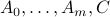A_0,ldots,A_m,C and vectors b_0,ldots,b_m,d . Precisely, we set b_i = log c_i , and A_i to be the matrices with rows 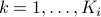$a_{ki}$ , k=1,ldots,K_i , i=0,ldots,m ; the matrix contains the vectors f_j as rows, j=1,ldots,p .

Example: Convex form of the water tank optimization problem.

CVX Syntax

With the above convex representation of a GP, We can directly invoke CVX with the logsumexp_sdp function. CVX knows it is convex. The extension ‘‘sdp’’ at the end of the function refers to the fact that the function is actually approximated via a technique based on semidefinite programming (SDP).

In CVX there is actually no need to transform the problem into the standard convex format. All you need to do is let CVX know that the problem is a GP. This is done by replacing the command cvx_begin with cvx_begin gp. This is illustrated here.