Linear Optimization
Definition and standard forms
Examples
Definition and standard forms
Definition
A linear optimization problem (or, linear program, LP) is one of the standard form:
![displaystylemin_x : f_0(x) ~:~ begin{array}[t]{l} f_i(x) le 0,quad i=1,cdots, m, Ax = b, quad i=1,cdots,p, end{array}](eqs/7020264096316324256-130.png)
where every function  is affine. Thus, the feasible set of an LP is a polyhedron.
Standard forms
Linear optimization problems admits several standard forms. One is derived from the general standard form:
where the inequalities are understood componentwise. Notice that the convention for componentwise inequalities differs from the one adopted in BV. I will reserve the symbol  or
or  for negative and positive semi-definiteness of symmetric matrices. The constant term
  in the objective function is, of course, immaterial.
Another standard form — used in several off-the-shelf algorithms — -is
We can always transform the above problem into the previous standard form, and vice-versa.
Examples
Piece-wise linear minimization
A piece-wise linear function is the point-wise maximum of affine functions, and has the form
for appropriate vectors  and scalars
  ,
,  . The (unconstrained) problem of minimizing the piece-wise linear function above is not an LP. However, its epigraph form:
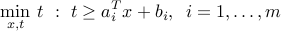
is.
 -norm regression
A related example involves the minimization of the -norm of a vector that depends affinely on the variable. This arises in regression problems, such as image reconstruction. Using a notation similar to the previous example, the problem has the form
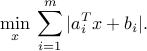
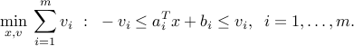
The problem is not an LP, but we can introduce slack variables and re-write the above in the equivalent, LP format:
Linear binary classification
|
|
A linear classifier, with a total of four errors on the training set. The sum of the lengths of the dotted lines (which correspond to classification errors) is the value of the loss function at optimum. |
Consider a two-class classification problem as shown above. Given  data points
  , each of which is associated with a label
  , the problem is to find a hyperplane that separates, as much as possible, the two classes.
The two classes are separable by a hyperplane  , where
  ,
,  , and
, and  , if and only if
  for
for  , and
, and 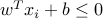 if
if  . Thus, the conditions on

ensure that the data set is separable by a linear classifier. In this case, the parameters  allow to predict the label associated to a new point
  , via
, via 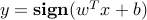 . The feasibility problem — finding that satisfy the above separability constraints — is an LP. If the data set is strictly separable (every condition in the above holds strictly), then we can re-scale the constraints and transform them into

In practice, the two classes may not be linearly separable. In this case, we would like to minimize, by proper choice of the hyperplane parameters, the total number of classification errors. Our objective function has the form
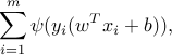
where  if
if  , and
, and  otherwise.
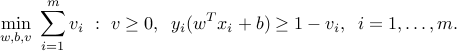
Unfortunately, the above objective function is not convex, and hard to minimize. We can replace it by an upper bound, which is called the hinge function,  . Our problem becomes one of minimizing a piece-wise linear ‘‘loss’’ function:
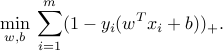
In the above form, the problem is not yet an LP. We may introduce slack variables to obtain the LP form:
The above can be seen as a variant of the separability conditions seen before, where we allow for infeasibilities, and seek to minimize their sum. The value of the loss function at optimum can be read from the figure: it is the sum of the lengths of the dotted lines, from data points that are wrongly classified, to the hyperplane.
Network flow
Consider a network (directed graph) having nodes connected by  directed arcs (ordered pairs
  ). We assume there is at most one arc from node
  to node
  , and no self-loops. We define the arc-node incidence matrix
  to be the matrix with coefficients
  if arc starts at node ,
  if it ends there, and otherwise. Note that the column sums of
  are zero:
  .
.
A flow (of traffic, information, charge) is represented by a vector  , and the total flow leaving node is then
 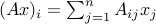 .
.
The minimum cost network flow problem has the LP form
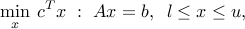
where  is the cost of flow through arc ,
  provide upper and lower bounds on and
  is an external supply vector. This vector may have positive or negative components, as it represents supply and demand. We assume that
  , so that the total supply equals the total demand. The constraint
  represents the balance equations of the network.
A more specific example is the max-flow problem, where we seek to maximize the flow between node  (the source) and node (the sink). It bears the form
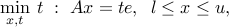
with  .
.
LP relaxation of boolean problems
A boolean optimization problem is one where the variables are constrained to be boolean. An example of boolean problem is the so-called boolean LP

Such problems are non-convex, and usually hard to solve. The LP relaxation takes the form

The relaxation provides a lower bound on the original problem:  . Hence, its optimal points may not be feasible (not boolean). Even though a solution of the LP relaxation may not necessarily be boolean, we can often interpret it as a fractional solution to the original problem. For example, in a graph coloring problem, the LP relaxation colors the nodes of the graph not with a single color, but with many.
Boolean problems are not always hard to solve. Indeed, in some cases, one can show that the LP relaxation provides an exact solution to the boolean problem, as optimal points turn out to be boolean. A few examples in this category, involving network flow problems with boolean variables:
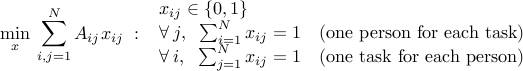
The weighted bipartite matching problem is to match
 people to tasks, in a one-to-one fashion. The cost of matching person to task is
  . The problem reads
The shortest path problem has the form

where stands for the incidence matrix of the network, and arcs with  form a shortest forward path between nodes and . As before the LP relaxation in this case is exact, in the sense that its solution is boolean. (The LP relaxation problem can be solved very efficiently with specialized algorithms.)