From Linear to Conic Optimization

Conic Optimization > LP | Overview | SOCP | SDP

From linear to conic
Tractable conic optimization

From linear to conic

The linear optimization model can be written in standard form as
min_x : c^Tx ~:~ Ax = b, ;; x ge 0,
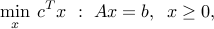
where we express the feasible set as the intersection of an affine subspace { x ::: Ax=b} , with the non-negative orthant, $mathbf{R}^n_{+}$ . One can think of the linear equality constraints, and the objective, as the part in the problem that involves the data (A,b,c) , while the sign constraints describe its structure.

With the advent of provably polynomial-time methods for linear optimization in the late 70’s, researchers tried to generalize the linear optimization model, in a way that retained the nice complexity properties of the linear model.

Early attempts at generalizing the above model focussed on allowing the linear map x rightarrow Ax to be nonlinear. Unfortunately, as soon as we introduce non-linearities in the equality constraints, the model becomes non-convex and potentially intractable numerically. Thus, modifying the linear equality constraints is probably not the right way to go.

Instead, one can try to modify the “structural” constraints $x in mathbf{R}_+^n$ . If one replaces the non-negative orthant with another set {cal K} , then we obtain a generalization of linear optimization. Clearly, we need {cal K} to be a convex set, and we can further assume it to be a cone (if not, we can always introduce a new variable and a new equality constraint in order to satisfy this condition). Hence the motivation for the so-called conic optimization model:
$min_x : c^Tx ~:~ Ax = b, ;; x in {cal K} ,$
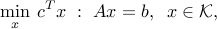
where {cal K} is a given convex cone.

The issue becomes then of finding those convex cones {cal K} for which one can adapt the efficient methods invented for linear optimization, to the conic problem above. A nice theory due to Nesterov and Nemirovski, which they developed in the late 80’s, allows to find a rich class of cones for which the corresponding conic optimization problem is numerically tractable. We refer to this class as tractable conic optimization.

Tractable conic optimization

The cones that are ‘‘allowed’’ in tractable conic optimization are of three basic types, and include any combination (as detailed below) of these three basic types. The three basic cones are

item The non-negative orthant, $mathbf{R}^n_+$ . (Hence, conic optimization includes linear optimization as a special case.)

The second-order cone, ${cal Q}^n := { (x,t) in mathbf{R}^{n}_+ ::: t ge |x|_2 }$ .
The semi-definite cone, ${cal S}_+^n = { X=X^T succeq 0}$ .

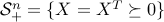A variation on the second-order cone, which is useful in applications, involves the rotated second-order cone $ (

{cal Q}_{rm rot}^n := { (x,y,z) in mathbf{R}^{n+2} ::: 2yz ge |x|_2^2, : y ge 0, : z ge 0}. ) We can easily convert the rotated second-order cone into the ordinary second-order cone representation, since the constraints , y ge 0 , z ge 0 , are equivalent to
$(y+z) ge left| begin{array}{c} (y-z) sqrt{2} : x end{array} right|_2.$

We can build all sorts of cones that are admissible for the tractable conic optimization model, using combinations of these cones. For example, in a specific instance of the problem, we might have constraints of the form
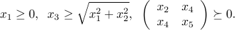
$x_1 ge 0, ;; x_3 ge sqrt{x_1^2+x_2^2}, ;; left(begin{array}{cc} x_2 & x_4 x_4 & x_5 end{array}right) succeq 0.$
The above set of constraints involves the non-negative orthant (first constraint), the second-order cone (second constraint), and the third, the semi-definite cone.

We can always introduce new variables and equality constraints, to make sure that the cone {cal K} is a direct product of the form ${cal K}_1 times ldots times {cal K}_m$ , where each ${cal K}_i$ is a cone of one of the three basic types above. In the example above, since the variable x_2 appears in two of the cones, we add a new variable x_6 and the equality constraint x_2 = x_6 . With that constraint, the constraint above can be written $x = (x_1,ldots,x_6) in {cal K}$ , where {cal K} is the direct product $mathbf{R}_+ times {cal Q}^2 times {cal S}_+^2$ .

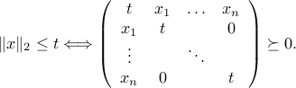
Note that the three basic cones are nested, in the sense that we can interpret the non-negative orthant as the projection of a direct product of second-order cones on a subspace (think of imposing x=0 in the definition of ${cal Q}^n$ ). Likewise, a projection of the semi-definite cone on a specific subspace gives the second-order cone, since
$|x|_2 le t Longleftrightarrow left(begin{array}{cccc} t & x_1 & ldots & x_n x_1 & t & & 0 vdots & & ddots & x_n & 0 & & t end{array}right) succeq 0.$
(The proof of this exercise hinges on the Schur complement lemma, see BV, pages 650-651.)