Semidefinite Optimization
Definitions and standard forms
Special cases
Examples
Definition and standard forms
Definition
We say that a problem is a semidefinite optimization problem (SDP) if it is a conic optimization problem of the form
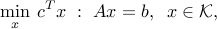
where the cone  is a product of semidefinite cones of given size. The decision variable
  contains elements of matrices, and the constraint
  imposes positive semi-definiteness on such matrices.
Standard form
Often, it is useful to think of as a matrix variable. The following standard form formalizes this.
First note that, without loss of generality, we may assume that  . Let us take an example with
  to illustrate why. Indeed, the condition that
  is the same as
  . Thus, by imposing that certain elements of the matrix
  be zero (those outside the diagonal blocks of size
  ), we can always reduce our problem to the case when the cone is the semidefinite cone itself, and the matrix variable is constrained to be block diagonal (with block sizes
  ,
,  ), and live in that cone.
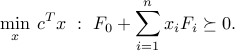
A standard form for the SDP model is thus

where 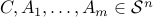 , and
, and  . (In the above, we have used the fact that a single affine equality constraint on a symmetric matrix variable can be represented as a scalar product condition of the form
  , for appropriate symmetric matrix
  and scalar
  .)
.)
Inequality form
An alternate standard form, called the inequality standard form, is
where matrices 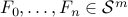 . The constraint in the above problem is called a linear matrix inequality (LMI). The above form is easily converted to the previous standard form (I suggest you try as an exercise).
Special cases
As discussed above, we can use the above formalism to handle multiple LMIs, using block-diagonal matrices. To illustrate this, we show that SDPs contain LPs as a special case. Indeed, the LP
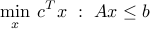
is equivalent to the SDP

where  is the
  -th row of . Thus, LPs are SDPs with a diagonal matrix in the LMIs.
Similarly, SDPs contain SOCPs, by virtue of the following result, already mentioned in XXX: for every  ,
,
Thus, a second-order cone constraint can be written as an LMI with an ‘‘arrow’’ matrix.
Examples
SDP relaxation of boolean problems
In lecture 5, we have seen LP relaxations for boolean LPs, which are LPs with the added non-convex requirement that the decision variable should be a boolean vector. This approach does not easily extend to the case when the problem involves quadratics.
To illustrate this, consider the max-cut problem. We are given a graph with vertices labeled  , with weights
  for every pair of vertices
  . We seek a cut (a subset
  of
of  ) such that the total weight of all the edges that leave is maximized. This can be expressed as the quadratic boolean problem
The problem is NP-hard. In 1995, Goemans and Williamson introduced an SDP relaxation (upper bound) of the problem, and showed that its value is at most within  of the optimal value of the combinatorial problem above, independent of problem size.
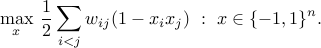
To explain the relaxation, let us embed the above problem into the more general problem of maximizing a given quadratic form over a boolean set:
where  is a given symmetric matrix. (As an exercise, try to cast the max-cut problem into the above formalism.)
We can express the problem as

Indeed, is feasible for the above if and only  for some
  , in which case
 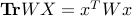 .
.
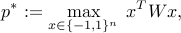
Relaxing (meaning: ignoring) the rank constraint leads to the upper bound  , where

The above is an SDP (in standard form). Nesterov has shown that, for arbitrary matrices  , the above relaxation is within
  of the true value, that is,
  .
.
Non-convex quadratic optimization
The approach used above can be applied to general non-convex quadratic optimization, which has the form

where  is the decision variable, and
  ’s are quadratic functions, of the form

with  ,
,  and
and  given. The above problem is not convex in general (we have not imposed positive semi-definiteness on the
  ’s).
’s).
We note that  , with
  the affine functions:

We can express the problem as

Dropping the rank constraint leads to an SDP relaxation (lower bound):

The above relaxation can be arbitrarily bad, but in some cases it is exact. For example, in the case of a single inequality constraint ( ), the SDP relaxation provides the exact value of the original non-convex problem.
%=== Optimization of ellipsoids.
%=== Polynomial optimization.
Stability analysis of uncertain dynamical systems. Consider a time-varying dynamical system of the form

with  the state vector, and
  . We assume that all is known about
  is that
  , with
  ,
,  given matrices. We say that the system is asymptotically stable if, for every initial condition
  , the resulting trajectory goes to zero:
  as
as  . Note that ascertaining asymptotic stability of the above ‘‘switched’’ system is hard in general, so we look for a tractable sufficient condition for asymptotic stability.
Let us denote by  the largest singular value norm. Clearly, if for every
  , we have
  for some
  , then
  , which shows that the state vector goes to zero at least as fast as
  . The norm condition ‘‘
 for every
  ’’ is conservative, since it implies that the state decreases monotonically.
To refine the norm-based sufficient condition for asymptotic stability, we can use scaling. For  a given invertible matrix, we define
  . In the new state space defined by
  , the state equations become
  , with
  . The asymptotic stability of the system is independent of the choice of , since
  converges to zero if and only if
  does. However, the norm-based sufficient condition for asymptotic stability is not independent of the choice of . Indeed, if we impose that condition on
  , we obtain
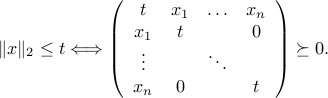
  . In turn, this condition writesfootnote{Here, we use the fact that for a matrix , the condition
  is equivalent to
  (try to show this).}
where  . (The original norm-based sufficient condition is recovered with
  .)
.)
We conclude that the existence of  such that

ensures the stability of the system, regardless of the choice of the trajectory of the matrix  . The above condition is an LMI in matrix variable
  .
.
Note that since for fixed  , the set
  is convex, requiring that it contains the finite set
  is the same as requiring that it contains its convex hull. So the above condition also ensures stability of the system, when is allowed to be any time-varying convex combination of the matrices
  , .
, .
Also, note that when  , the above condition turns out to be exact, and equivalent to the condition that all the eigenvalues of the matrix lie in the interior of the unit circle of the complex plane. This is the basic result of the so-called Lyapunov asymptotic stability theorem for linear systems.