A Simple Convex Optimization Algorithm
In this section, we aim to show that convex optimization is a computationally tractable problem, by presenting a simple method for general-purpose convex optimization, the subgradient method.
The subgradient method
Convergence analysis and complexity
Projected subgradient method
The subgradient method
The subgradient method is a simple algorithm for minimizing a non-differentiable convex function, and more generally, solving convex optimization problems. Its complexity in terms of problem size is very good (each iteration is cheap), but in terms of accuracy, very poor (the algorithm typically requires thousands or millions of iterations). The convergence analysis of the algorithm has an important theoretical consequence: it shows that convex optimization is essentially ‘‘tractable’’, provided we can compute subgradients of the objective and constraints functions efficiently.
The method is part of a large class of methods known as first-order methods, which are based on subgradients or closely related objects. In constrast, second-order methods typically use Hessian information; each iteration is expensive (both in flops and memory) but convergence is obtained very quickly.
Setup
The setup is as follows. Let  be a convex function. We seek to solve the uconstrained problem
To minimize  , the subgradient method described below uses only subgradient information at every step.
Now consider the convex, inequality constrained problem:

We can formulate this as an unconstrained problem of minimizing the function  , with
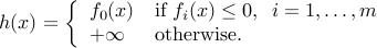
Certainly, is not differentiable, but it is convex. So we can apply the subgradient method for unconstrained minimization to this function.
Algorithm
The algorithm proceeds as follows:

Here,  is the
  -th iterate,
  is any subgradient of
at , and
is any subgradient of
at , and  is the -th step size. Thus, at each iteration of
the subgradient method, we take a step in the direction of a
negative subgradient. Since this is not a descent method (the objective is not guaranteed to decrease at each step), we must
keep track of the best solution seen so far, via the values
is the -th step size. Thus, at each iteration of
the subgradient method, we take a step in the direction of a
negative subgradient. Since this is not a descent method (the objective is not guaranteed to decrease at each step), we must
keep track of the best solution seen so far, via the values
We will also denote  .
.
Convergence analysis and complexity
To analyze the convergence, we make the following assumptions:
 is finite and attained
There is a constant
 such that, for every
  , and every
  ,
we have
,
we have  .
.There is a large enough constant
 such that
 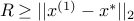 .
.
Now let  be any minimizer of . We have
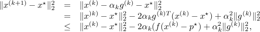
where we have used the subgradient inequality:

Applying this recursively, we get

By definition of  , we have
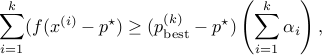
which yields
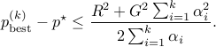
This shows that
For constant step sizes (
 for every ), the condition
  guarantees that
  .
.For constant step length (
 ), the condition
  guarantees that .
Complexity
The convergence analysis result (ref{eq:conv-anal-L19}) depends on the choice of the step size rule. Which rule is optimal for this bound? The problem of minimizing the upper bound above is convex and symmetric (the function does not change when we exchange variables). Hence, the optimal  ’s are all equal at optimum, to a number
  . With this choice of step length rule, the number of iterations needed to achieve
  -sub-optimality, as predicted by the analysis, is
  . The dependence on is now
  , which is very slow. Interior-point methods alluded to earlier typically behave in
  ), but they do not apply to general convex problems, only to a special class.
The above discusses the dependence of complexity on the accuracy . The complexity depends on problem size as well, and more generally, on the structure of the function involved, via the need to compute subgradients at each step, and also the parameters and .
Example: We seek to find a point in a given intersection of closed convex sets,

We formulate this problem as minimizing , where

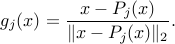
Let  the projection operator on
  , and let
be the corresponding distance function. Thus,  achieves the
minimum value of
achieves the
minimum value of  . Then, a subgradient of at is
Projected subgradient method
One extension of the subgradient method for solving constrained
optimization problems, is the projected subgradient method. We consider the problem
where  is a convex set, which can be defined by a set of
inequality constraints. The projected subgradient method uses the
iteration
is a convex set, which can be defined by a set of
inequality constraints. The projected subgradient method uses the
iteration
where  is projection on , and
  is any subgradient of
at
is any subgradient of
at  .
.
Example:
Let  ,
,  , with
  ,
,  full rank (hence,
  ). We consider the problem
The projection on the affine space  is
is
The subgradient iterations are given by:

where we have exploited the fact that the operator  is linear.