Convex Functions
Domain of a function
Definition of convexity
Alternate characterizations of convexity
Operations that preserve convexity
Subgradients
Domain of a function
The domain of a function  is the set
  over which
  is well-defined, in other words:
(
is well-defined, in other words:
(
{bf dom}f :={ x in mathbf{R}^n: -infty < f(x) < +infty}. ) Here are some examples:
The function with values
 has domain
  .
.The function with values
 has domain
  (the set of positive-definite matrices).
Definition of convexity
A function  is convex if
 is convex;
 and
and ![forall, lambdain [0, 1]](eqs/8434653919099798392-130.png) ,
,  .
Note that the convexity of the domain is required. For example, the function
.
Note that the convexity of the domain is required. For example, the function  defined as
![f(x) = left{ begin{array}{ll} x & mbox{if } x notin [-1,1] +infty & mbox{otherwise} end{array}right.](eqs/3707423515173210456-130.png)
is not convex, although is it linear (hence, convex) on its domain![]-infty,-1)cup(1,+infty[](eqs/4406577851778482381-130.png) .
.
We say that a function is concave if  is convex.
Here are some examples:
The support function of a given set
 , which is defined as
  , is convex for any set
  .
.The indicator function of a given set
, defined as
is convex if and only if is convex.
A norm is a convex function that is positively homogeneous (
 for every
  ,
,  ), and positive-definite (it is non-negative, and zero if and only if its argument is).
 The quadratic function
 , with
  , is convex. (For a proof, see later.)
The function
defined as  for
for  and
and  is convex.
The function
defined as  for every
  is not convex; but if we modify to take the value
  on the set of non-positive real numbers, then it is convex.
end{itemize}
on the set of non-positive real numbers, then it is convex.
end{itemize}
Alternate characterizations of convexity
Let . The following are equivalent conditions for to be convex.
Epigraph condition:
is convex if and only if its epigraph

is convex. We can us this result to prove for example, that the largest eigenvalue function , which to a given
  symmetric matrix
  associates its largest eigenvalue, is convex, since the condition
  is equivalent to the condition that
  .
.
Restriction to a line: The function
is convex if and only if its restriction to any line is convex, meaning that for every  , and
, and  , the function
  is convex.
For example, the function  is convex. (Prove this as an exercise.) You can also use this to prove that the quadratic function is convex if and only if
  .
.
First-order condition: If
is differentiable (that is,  is open and the gradient exists everywhere on the domain), then is convex if and only if

The geometric interpretation is that the graph of is bounded below everywhere by anyone of its tangents.
Second-order condition: If
is twice differentiable, then it is convex if and only if its Hessian  is positive semi-definite everywhere. This is perhaps the most commonly known characterization of convexity, although it is often hard to check.
For example, the function  with domain
  , is convex. (Check this!) Other examples include the log-sum-exp function,
  , and the quadratic function alluded to above.
Operations that preserve convexity
The nonnegative weighted sum of convex functions is convex.
The composition with an affine function preserves convexity: if
 ,
,  and
and  is convex, then the function
  with values
  is convex.
The pointwise maximum of a family of convex functions is convex: if
 is a family of convex functions index by
  , then the function
is convex. For example, the dual norm
is convex, as the maximum of convex (in fact, linear) functions (indexed by the vector ). Another example is the largest singular value of a matrix
  :
:  . Here, each function (indexed by
  )
)  is convex, since it is the composition of the Euclidean norm (a convex function) with an affine function
  . Also, this can be used to prove convexity of the function we introduced in lecture 2,
![|x|_{1,k} := sum_{i=1}^k |x|_{[i]} = max_{u} : u^T|x| ~:~ sum_{i=1}^n u_i = k, ;; uin{0,1}^n,](eqs/3517482603802280937-130.png)
where we use the fact that for any feasible for the maximization problem, the function
  is convex (since
  ).
).If
is a convex function in  , then the function
  is convex. (Note that joint convexity in
  is essential.)
 If
is convex, its perspective  with domain
  , is convex. You can use this to prove convexity of the function , with domain .
The composition with another function does not always preserve convexity. However, if the functions
 ,
,  are convex and
  is convex and non-decreasing in each argument, with
  , then
  is convex.
For example, if  ’s are convex, then
  also is.
Subgradients
Definition
Let  be a convex function. The vector
  is a subgradient of
  at
at  if the subgradient inequality:
holds for every . The subdifferential of at , denoted  , is the set of such subgradients at .
 is convex, closed, never empty on the relative interiorfootnote{The relative interior of a set is the interior of the set, relative to the smallest affine subspace that contains it.} of its domain.
if
is differentiable at , then the subdifferential is a singleton:
=  .
.
For example, consider  for
for  . We have
![partial f(x) = left{ begin{array}{ll} {-1} & mbox{if } x <0, [-1,1] & mbox{if } x = 0, {+1} & mbox{if } x >0. end{array}right.](eqs/3671723617860281829-130.png)
Constructing subgradients
One of the most important rules for contructing a subgradient is based on the following rule.
Weak rule for point-wise supremum: if  are differentiable and convex
functions that depend on a parameter
are differentiable and convex
functions that depend on a parameter  , with
  an arbitrary set, then
is possibly non-differentiable but convex.
If  is such that
  , then a subgradient of at is
simply any element in
, then a subgradient of at is
simply any element in  .
.
Example: maximum eigenvalue.
For  , define
 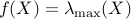 to be the largest eigenvalue of ( is real valued
since is symmetric). A subgradient of at can be found
using the following variational (that is, optimization-based)
representation of
to be the largest eigenvalue of ( is real valued
since is symmetric). A subgradient of at can be found
using the following variational (that is, optimization-based)
representation of  :
:
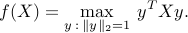
Any unit-norm eigenvector  of corresponding to the largest eigenvalue
achieves the maximum in the above. Hence, by the weak rule above, a subgradient of
at is given by a gradient of the function
of corresponding to the largest eigenvalue
achieves the maximum in the above. Hence, by the weak rule above, a subgradient of
at is given by a gradient of the function  ,
which is
,
which is  .
.