Convex Problems

Mathematical programming problems
Convex optimization problems
Optimality
Equivalent problems
Complexity

Mathematical programming problems

Definition

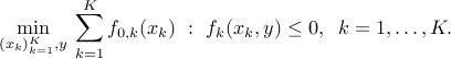
A mathematical programming problem is one of the form
$p^ast := min_x : f_0(x) mbox{ subject to } f_i(x) le 0, ;; i=1,ldots, m.$

The term “programming” (or “program”) does not refer to a computer code. It is used mainly for historical purposes. A more rigorous (but less popular) term is “optimization problem”. The term “subject to” is often replaced by a colon.

By convention, the quantity p^ast

is set to

if the problem is not feasible. The optimal value can also assume the value -infty

, in which case we say that the problem is unbounded below. An example of a problem that is unbounded below is an unconstrained problem with f_0(x) = -log x

, with domain $mathbf{R}_{++}$ .

{cal X} = left{ x in mathbf{R}^n : f_i(x) le 0, ;; i=1,ldots, m right} ) is called the feasible set. Any x in {cal X}

is called feasible (with respect to the specific optimization problem at hand).

Alternate representations

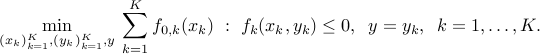
Sometimes, the model is described in terms of the feasible set, as follows:
$min_{x in {cal X}} : f_0(x) .$
The representation is not strictly equivalent to the more explicit form (ref{eq:math-program-CVXPBS}), since the set {cal X}

may have several equivalent representations in terms of explicit constraints. (Think for example about a polytope described by its vertices or as the intersection of half-spaces.)

Also, sometimes a maximization problem is considered:
$p^ast = max_{x in {cal X}} : f_0(x).$
Of course, we can always change the sign of f_0

and transform the maximization problem into a minimization one. For maximization problem, the optimal value p^star

is set by convention to -infty

if the problem is not feasible.

Feasibility problems

In some instances, we do not care about any objective function, and simply seek a feasible point. This so-called feasibility problem can be formulated in the standard form, using a zero (or constant) objective.

Convex optimization problems

Standard form

The problem
$displaystylemin_x : f_0(x) ~:~ begin{array}[t]{l} f_i(x) le 0,quad i=1,cdots, m, Ax = b, quad i=1,cdots,p, end{array}$
is called a convex optimization problem if the objective function f_0

is convex; the functions defining the inequality constraints f_i

are convex; and $A in mathbf{R}^{p times n}$ , $b in mathbf{R}^p$ define the affine equality constraints. Note that, in the convex optimization model, we do not tolerate equality constraints unless they are affine.

Optimality

Local and global optima

A feasible point $x^ast in {cal X}$ is a globally optimal (optimal for short) if f_0(x) = p^ast

A feasible point $x^ast in {cal X}$ is a locally optimal if there exist R>0

such that

equals the optimal value of problem (ref{eq:convex-pb-L4}) with the added constraint |x-x^ast| le R

. That is, x^ast

solves the problem ‘‘locally’’.

Indeed, let x^ast

be a local minimizer of f_0

on the set {cal X}

, and let

. By definition, $x^ast in {bf dom} f_0$ . We need to prove that f_0(y) ge f_0(x^ast) = p^ast

. There is nothing to prove if f_0(y) = +infty

, so let us assume that $y in {bf dom} f_0$ . By convexity of f_0

and

, we have $x_theta := theta y + (1-theta) x^ast in {cal X}$ , and:
f_0(x_theta) - f_0(x^ast) le theta (f_0(y) - f_0(x^ast)).

Since

is a local minimizer, the left-hand side in this inequality is nonnegative for all small enough values of theta > 0

. We conclude that the right hand side is nonnegative, i.e., f_0(y) ge f_0(x^ast)

, as claimed.

Optimal set

The optimal set, ${cal X}^{rm opt}$ , is the set of optimal points. This set may be empty: for example, the feasible set may be empty. Another example is when the optimal value is only reached in the limit; think for example of the case when n=1

, and there are no constraints.

{cal X}^{rm opt} = left{ x in mathbf{R}^n : f_0(x) le p^ast, ;; x in {cal X} right} . )

Optimality condition

When

is differentiable, then we know that for every $x,y in {bf dom} f_0$ ,
f_0(y) ge f_0(x) + nabla f_0(x) ^T (y-x).

Then

is optimal if and only if
$forall : y in {cal X} ~:~ nabla f_0(x) ^T (y-x) ge 0 .$
If nabla f_0(x) ne 0

, then it defines a supporting hyperplane to the feasible set at

Equivalent problems

We can transform a convex problem into an equivalent one via a number of transformations. Sometimes the transformation is useful to obtain an explicit solution, or is done for algorithmic purposes. The transformation does not necessarily preserve the convexity properties of the problem. Here is a list of transformations that do preserve convexity.

Epigraph form

Sometimes it is convenient to work with the equivalent epigraph form:
$min_{(x,t)} : t ~:~ t ge f_0(x), ;; x in {cal X},$
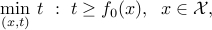
in which we observe that we can always assume the cost function to be differentiable (in fact, linear), at the cost of adding one scalar variable.

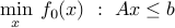
Implicit constraints

Even though some problems appear to be unconstrained, they might contain implicit constraints. Precisely, the problem above has an implicit constraint x in {cal D}

, where

is the problem’s domain (

{cal D} := {bf dom} f_0 bigcap_{i=1}^m {bf dom} f_i . ) For example, the problem
$min_x : c^Tx - sum_{i=1}^m log (b_i-a_i^Tx),$
where $c in mathbf{R}^n$ , $b in mathbf{R}^m$ and a_i^T

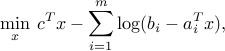
’s are the rows of $A in mathbf{R}^{m times n}$ , arises as an important sub-problem in some linear optimization algorithms. This problem has the implicit constraint that

should belong to the interior of the polyhedron {cal P} = { x ::: Ax le b }

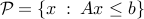Making explicit constraints implicit

The problem in standard form can be also written in a form that makes the constraints that are explicit in the original problem, implicit. Indeed, an equivalent formulation is the unconstrained convex problem
min_x : f(x)

where

is the sum of the original objective and the indicator function of the feasible set {cal X}

:
$f(x) = f_0(x) + mathbf{1}_{cal X}(x) = left{ begin{array}{ll} f_0(x) & x in {cal X} +infty &x notin {cal X}. end{array}right.$
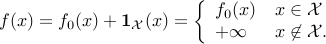
In the unconstrained above, the constraints are implicit. One of the main differences with the original, constrained problem is that now the objective function may not be differentiable, even if all the functions f_i

’s are.

A less radical approach involves the convex problem wih one inequality constraint
$min_x : f_0(x) ~:~ Ax= b, ;; g(x) := max_{1 le i le m} : f_i(x) le 0,$
which is equivalent to the original problem. In the above formulation, the structure of the inequality constraint is made implicit. Here, the reduction to a single constraint has a cost, since the function

may not be differentiable, even though all the f_i

’s are.

The above transformations show the versatility of the convex optimization model. They are also useful in the analysis of such problems.

Equality constraint elimination

We can eliminate the equality constraint Ax = b

, by writing them as x = x_0 + Nz

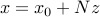, with

a particular solution to the equality constraint, and the columns of

span the nullspace of

. Then we can rewrite the problem as one without equality constraints:
min_z : f_0(Nz+x_0) ~:~ f_i(Nz+x_0) le 0, ;; i=1,ldots,m.

This transformation preserves convexity of the the function involved. In practice, it may not be a good idea to perform this elimination. For example, if

is sparse, the original problem has a sparse structure that may be exploited by some algorithms. In contrast, the reduced problem above does not inherit the sparsity characteristics, since in general the matrix

is dense.

Introducing equality constraints

We can also introduce equality constraints in the problem. There might be several justifications for doing so: to reduce a given problem to a standard form used by off-the-shelf algorithms, or to use in decomposition methods for large-scale optimization.

The following example shows that introducing equality constraint may allow to exploit sparsity patterns inherent to the problem. Consider
$min_{(x_k)_{k=1}^K,y} : sum_{k=1}^K f_{0,k}(x_k)~:~ f_k(x_k,y) le 0, ;; k=1,ldots,K.$
In the above the objective involves different optimization variables, which are coupled via the presence of the ‘‘coupling’’ variable

in each constraint. We can introduce

variables and rewrite the problem as
$min_{(x_k)_{k=1}^K,(y_k)_{k=1}^K,y} : sum_{k=1}^K f_{0,k}(x_k)~:~ f_k(x_k,y_k) le 0, ;; y = y_k, ;; k=1,ldots,K.$
Now the objective and inequality constraints are all independent (they involve different optimization variables). The only coupling constraint is now an equality constraint. This can be exploited in parallel algorithms for large-scale optimization.

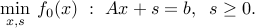
Slack variables

Sometimes it is useful to introduce slack variables. For example, the problem with affine inequalities
min_x : f_0(x) ~:~ Ax le b

can be written
$min_{x,s} : f_0(x) ~:~ Ax + s = b, ;; sge 0 .$

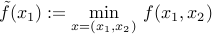
Minimizing over some variables

We may ‘‘eliminate’’ some variables of the problem and reduce it to one with fewer variables. This operation preserves convexity. Specifically, if

is a convex function of the variable $x in mathbf{R}^n$ , and

is partitioned as x=(x_1,x_2)

, with $x_i in mathbf{R}^{n_i}$ , i=1,2

, then the function
$tilde{f}(x_1) := min_{x=(x_1,x_2)} : f(x_1,x_2)$
is convex (look at the epigraph of this function). Hence the problem of minimizing

can be reduced to one involving x_1

only:
$min_{x_1} : tilde{f}(x_1).$
The reduction may not be easy to carry out explicitly.

Here is an example where it is: consider the problem
$min_{x=(x_1,x_2)} : x^TQx ~:~ A x_1 le b$
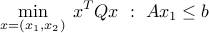
where
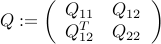
$Q := left( begin{array}{cc} Q_{11} & Q_{12} Q_{12}^T & Q_{22} end{array} right)$
is positive semi-definite, $Q_{22}$ is positive-definite, and $Q_{ij} in mathbf{R}^{n_i times n_j}$ , i,j=1,2

. Since

, the above problem is convex. Furthermore, since the problem has no constraints on x_2

, it is possible to solve for the minimization with respect to x_2

analytically. We end up with
$min_{x_1} : x_1^Ttilde{Q}x_1 ~:~ Ax_1 le b$
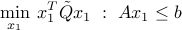
with 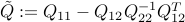$tilde{Q} := Q_{11} - Q_{12} Q_{22}^{-1} Q_{12}^T$ . From the reasoning above, we infer that

is positive semi-definite, since the objective function of the reduced problem is convex.

Complexity

Complexity of an optimization problem refers to the difficulty of solving the problem on a computer. Roughly speaking, complexity estimates provide the number of flops needed to solve the problem to a given accuracy of the objective epsilon

. That problem is usually expressed in terms of the problem size, as well as the accuracy epsilon

The complexity usually refers to a specific method to solve the problem. For example, we may say that solving a dense linear optimization problem to accuracy epsilon

with

variables and constraints using an ‘‘interior-point’’ methodfootnote{This term refers to a class of methods that are provably efficient for a large class of convex optimization problems.} grows as O(n^3 log(1/epsilon))

The complexity of an optimization problem also depends on its structure. Two seemingly similar problem may require a widely different computational effort to solve. Some problems are “NP-hard”, which roughly means that they cannot be solved in reasonable time on a computer. As an example, the quadratic programming problem (ref{eq:quad-prob-L1}) seen above is “easy” to solve, however the apparently similar problem obtained by allowing

to have negative eigenvalues is NP-hard.

In the early days of optimization, it was thought that linearity was what distinguished a hard problem from an easy one. Today, it appears that convexity is the relevant notion. Roughly speaking, a convex problem is easy. In the next section, we will refine this statement.