Project 4: Auto-Stitching Photo Mosaics
Project Overview
The aim of the project is to take a series of related photographs with overlapping details and
to "stitch" them together into one photo mosaic. Our initial approach involved assigning correspondences
manually between every image (as we did in Project 3) to instantiate
the merge. As this process is tedious, we will also explore strategies that allows for selecting keypoints automatically.
Let's explore!
Project Link
Phase A: Image Warping and Mosaicing
The main goal of this phase was to demonstrate how the homography transformation can allow one to warp images and create mosaics by manually stitch two different photos together with pre-defined keypoints.Part 1: Shoot the Pictures
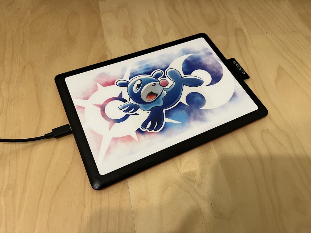
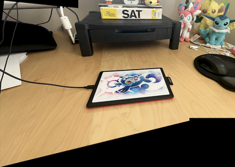
In order to observe the effects of homography, we need some data to work with! Listed below are images and their manually-selected keypoints that will be utilized during this phase.
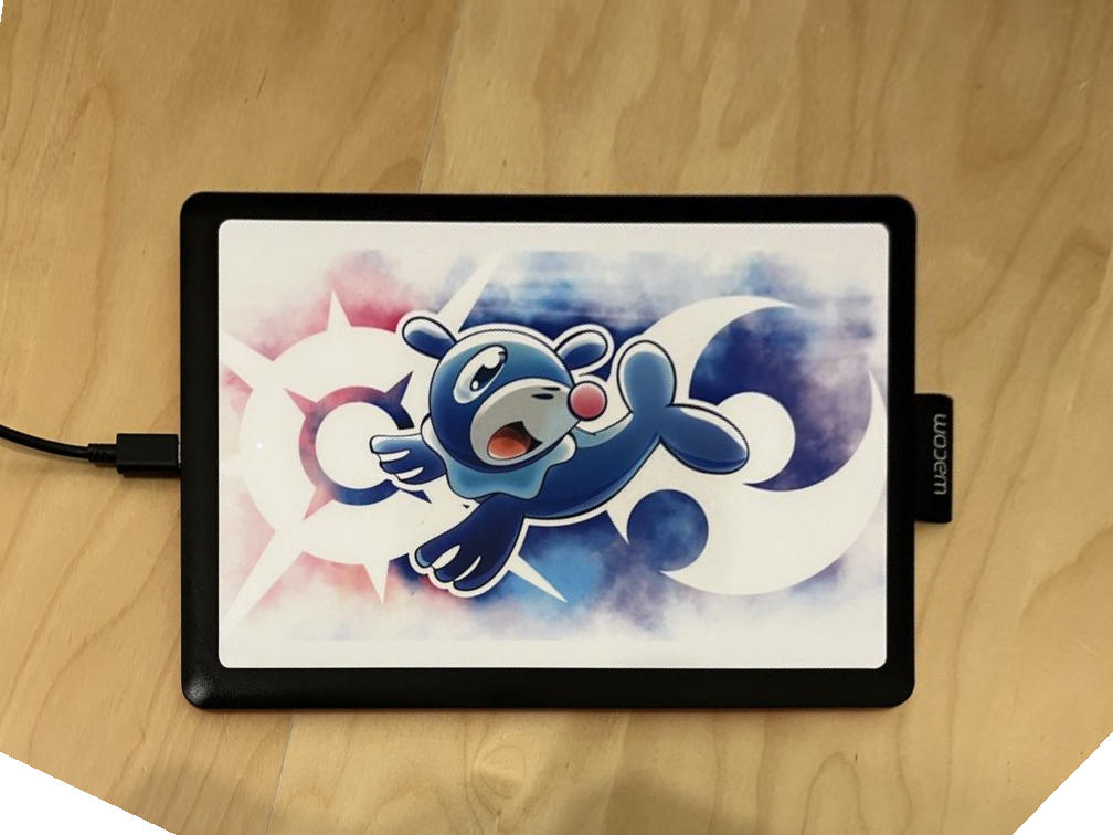
Tablet Cover
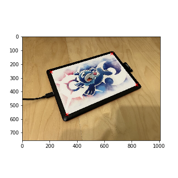
Tabler Cover (Keypoints)
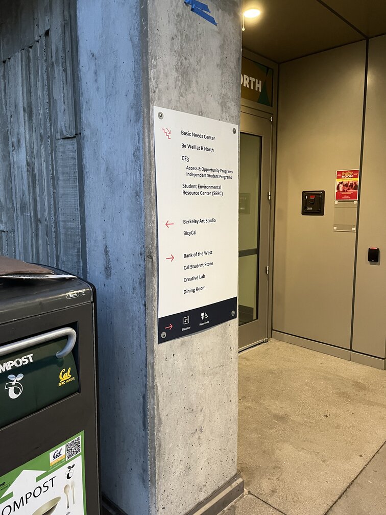
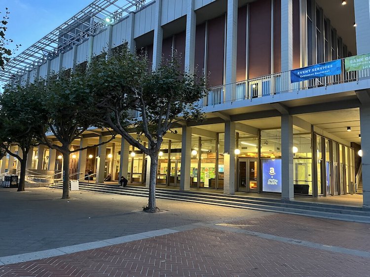
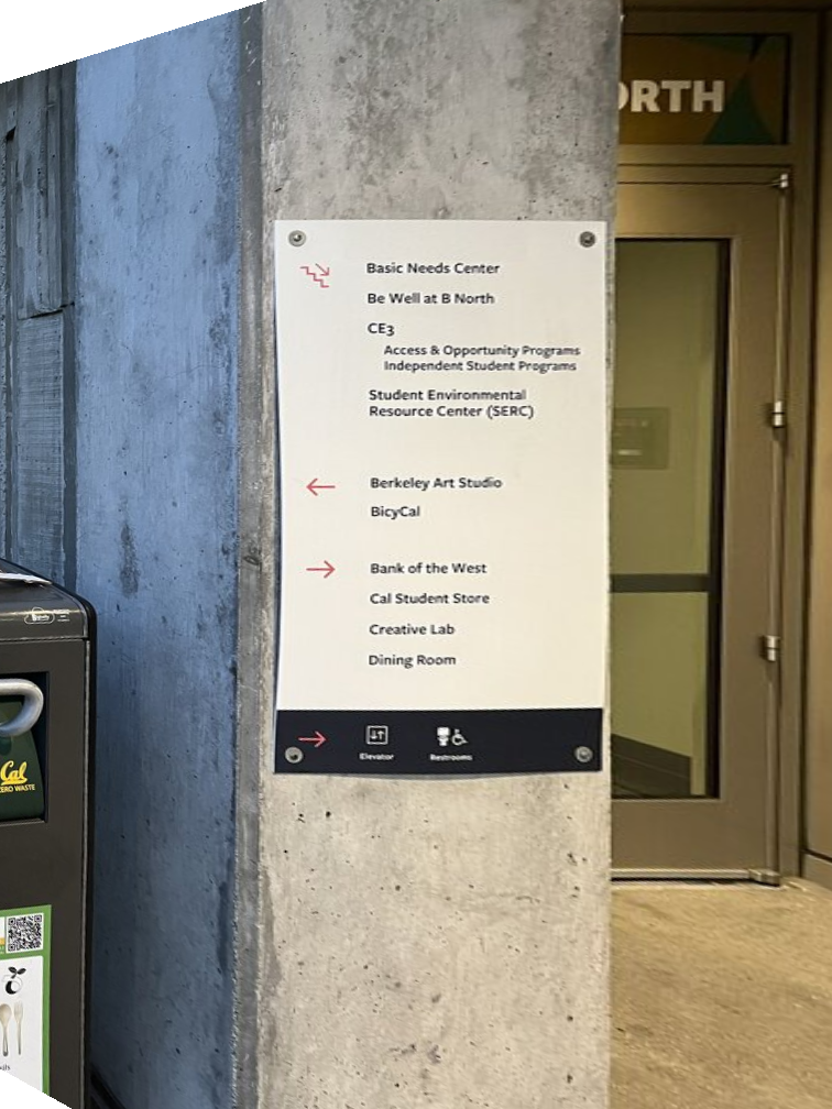
MLK Sign
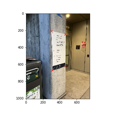
MLK Sign (Keypoints)
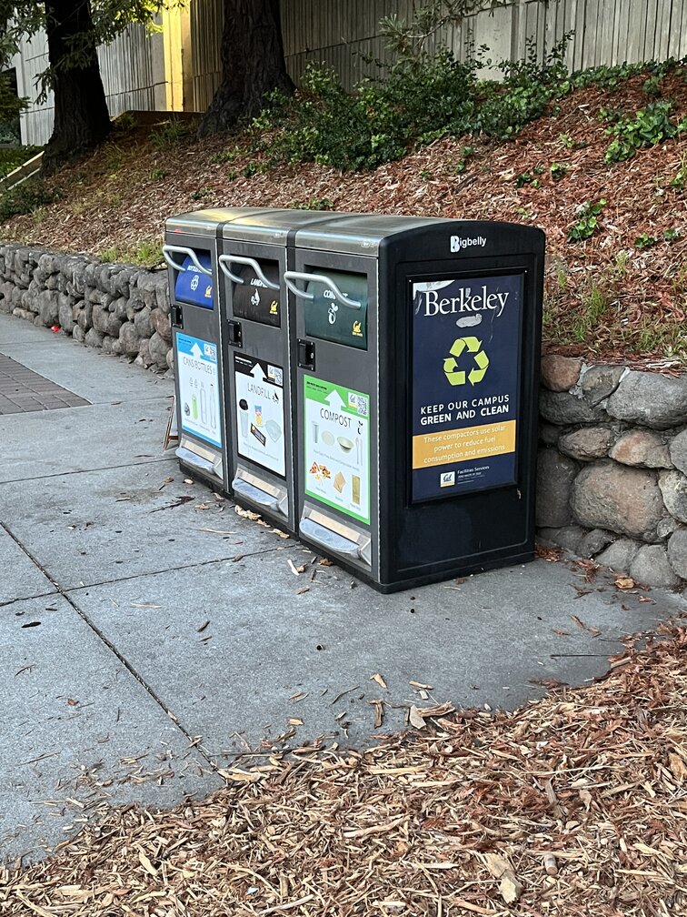
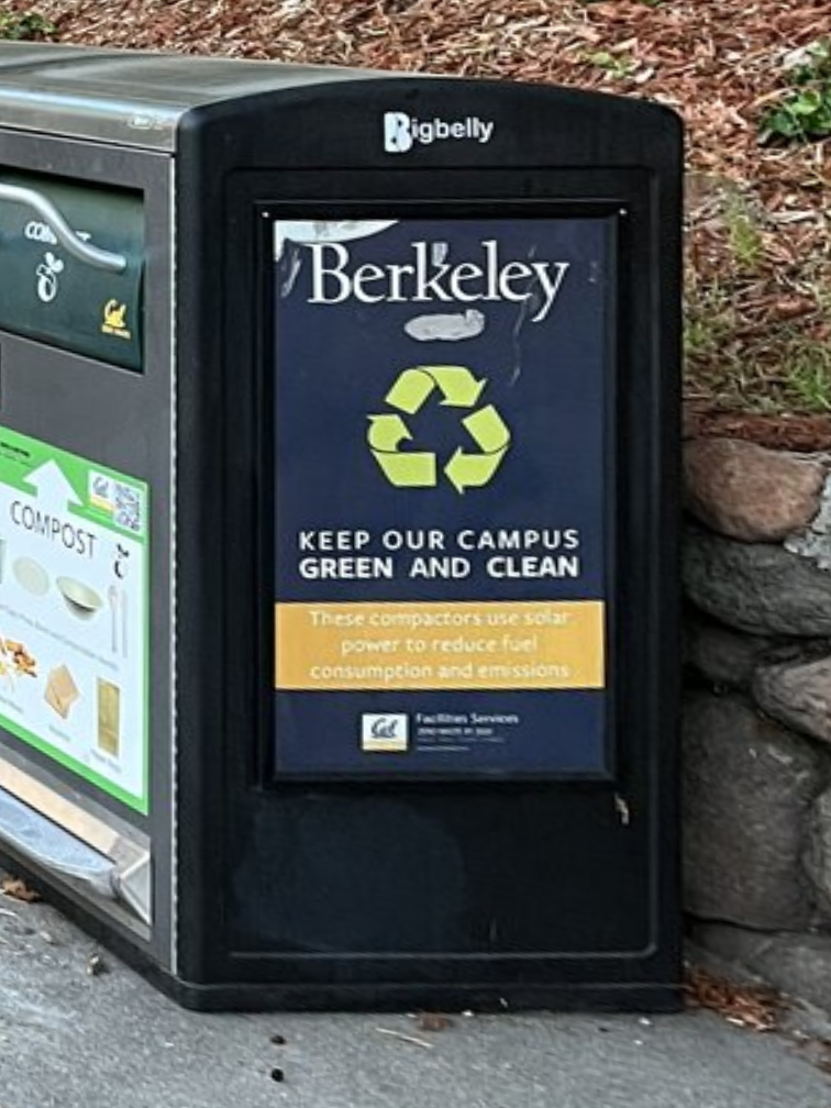
Berkeley Trashcan
Berkeley Trashcan (Keypoints)
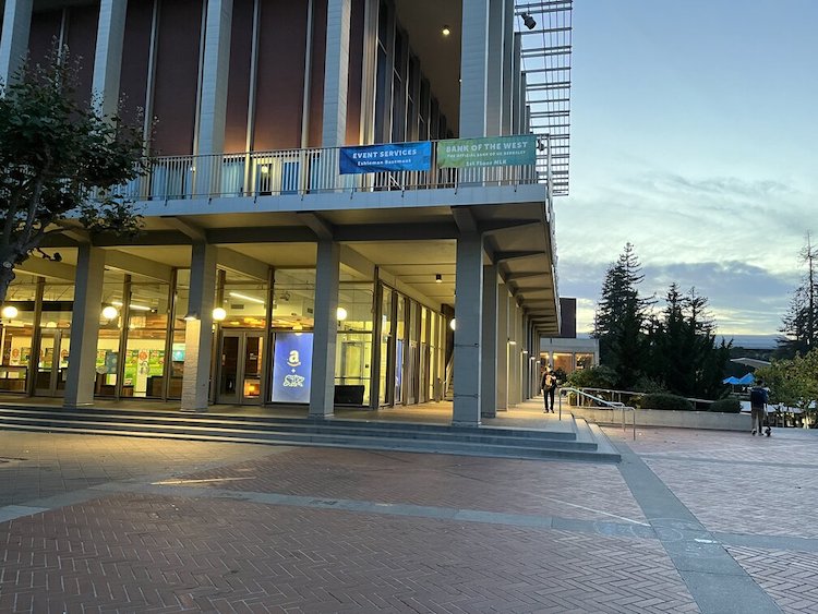
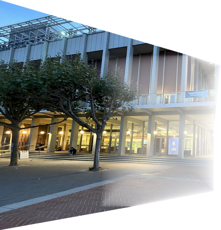
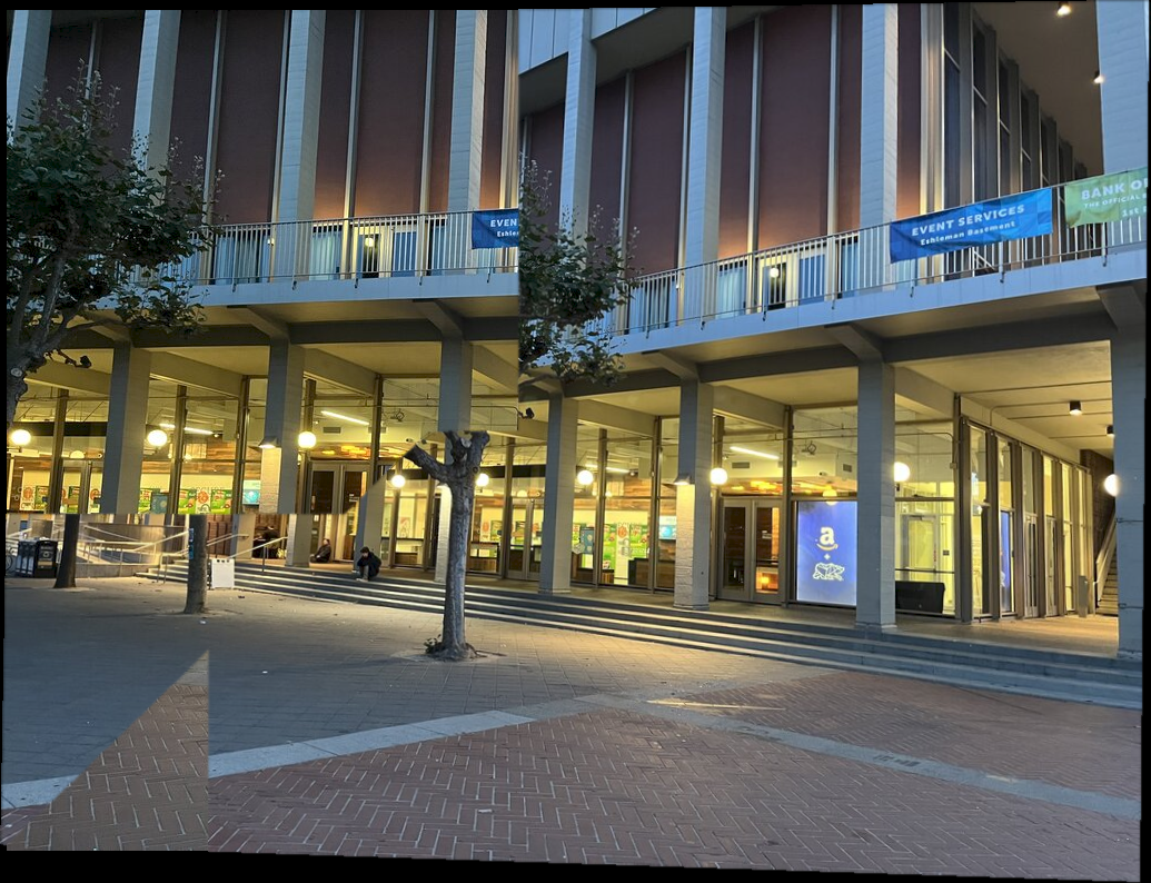
Amazon Locker (Left)
Amazon Locker (Left) (Keypoints)

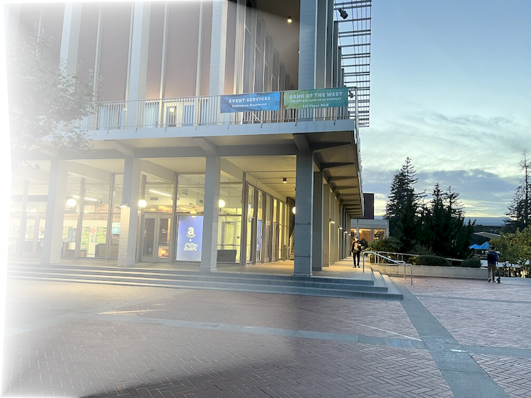
Amazon Locker (Right)
Amazon Locker (Right) (Keypoints)

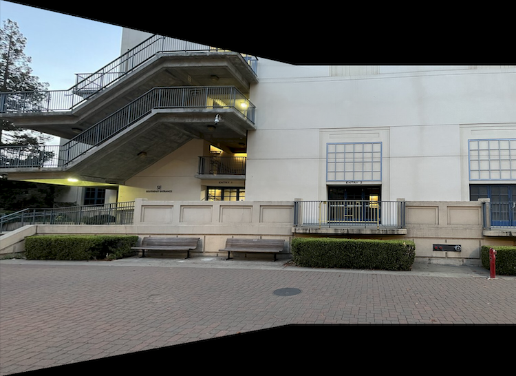
Haas Pavilion (Left)
Haas Pavilion (Left) (Keypoints)
Haas Pavilion (Right)
Haas Pavilion (Right) (Keypoints)
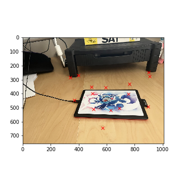
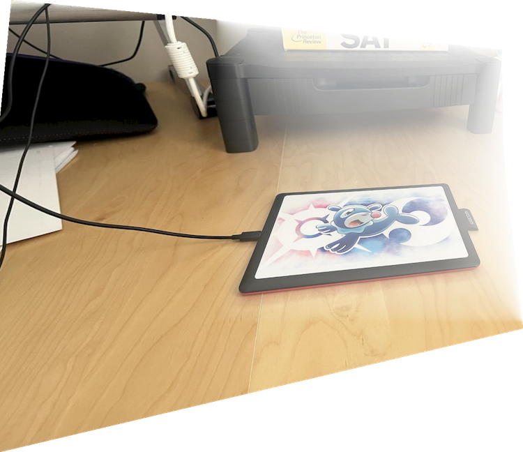
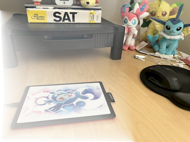
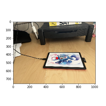
Tablet (Left)
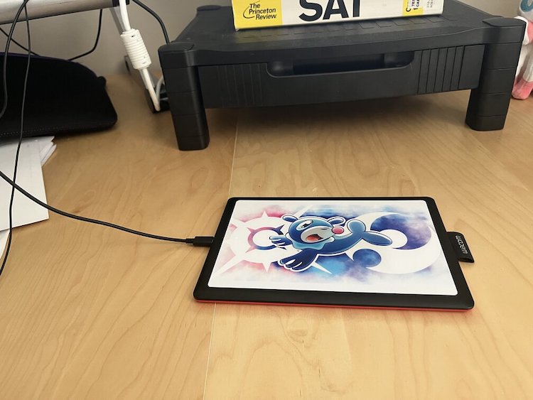
Tablet (Left) (Keypoints)
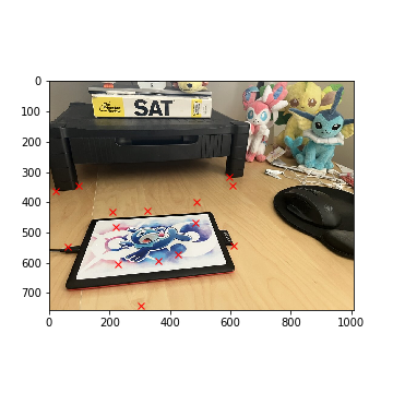
Tablet (Right)
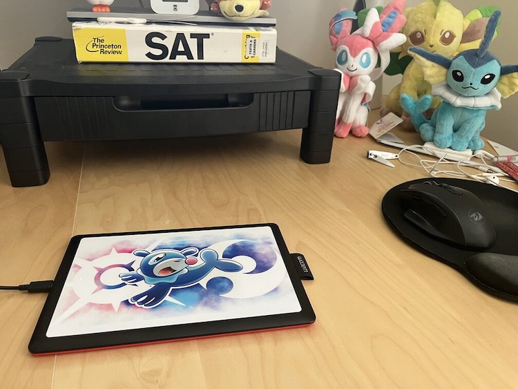
Tablet (Right) (Keypoints)
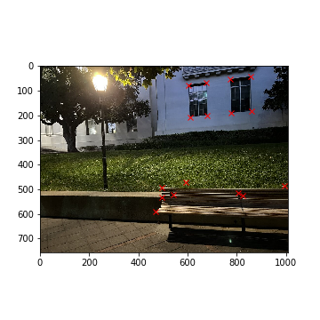
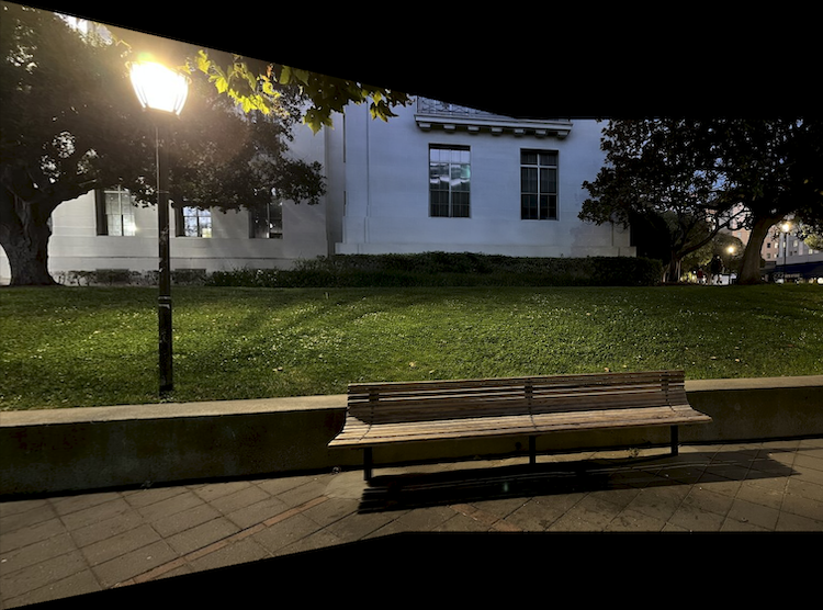
Bench (Left)
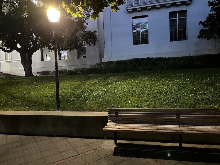
Bench (Left) (Keypoints)
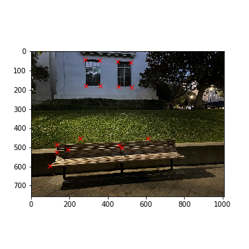
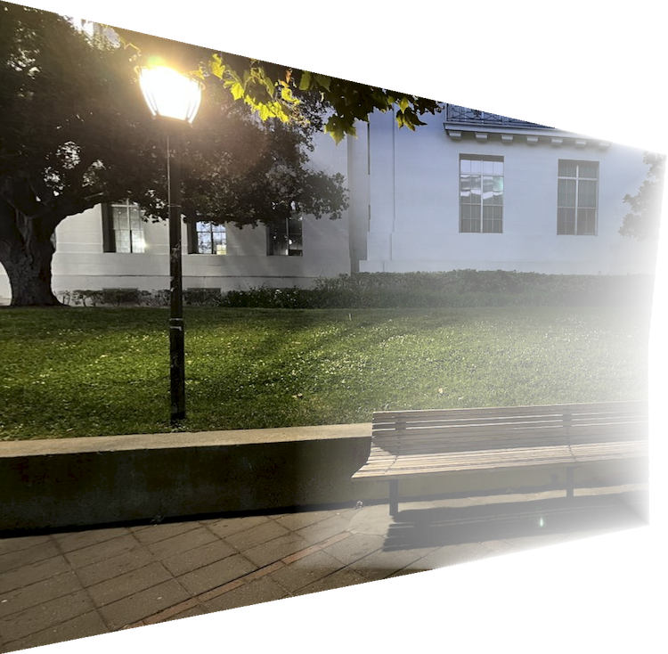
Bench (Right)
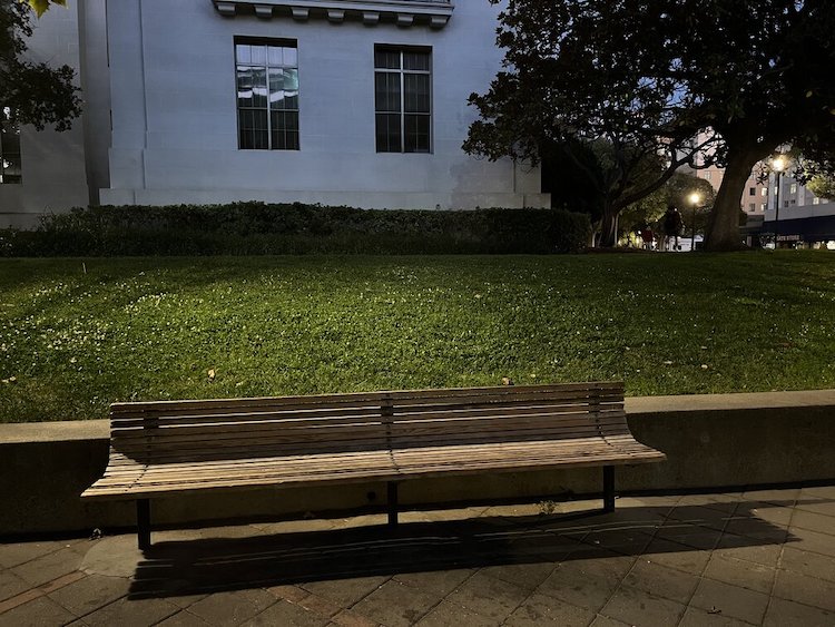
Bench (Keypoints)
Part 2: Recover Homographies
Next up, we need to establish a method that can define a homography matrix to map between two different set of keypoints.
Homography can be thought of as a projective transformation, where one can move the target image in any direction or angle
(in other words, 8 degrees of freedom). The homography matrix H is defined below: (where Hp = p'):
Note: to recover the coordinate (x', y') from p', divide wx' and wy' by w.
Given this matrix, we have 8 unknowns we need to solve; therefore at least 4 known keypoints are required to solve the system.
After rearranging some terms, we yield the following systems of equations to solve for the components of H given at
least keypoint 4 pairs:
Solving for [a, b, c, d, e, f, g, h]T allows us to construct the homography matrix. Note that providing more than
4 points creates an overdetermined system (more equations than unknowns) - as such, we can use least squares to solve this system.
Part 3: Warping Images + Image Rectification
After obtaining a desired transformation matrix H between two correspondences, we can warp the first image into the second
image. This process is similar to what was done in
Project 3: after defining the bounds of our destination image D based on H, we can iterate through every point p' in D,
find the corresponding point p = H-1 @ p' in the source image, then interpolate the color of p' from p using the
interp2d Scipy package.
To test our homography matrix, I took a few images from a slanted angle and transformed them into a "frontal-parallel" view by warping the image into a
pre-defined set of keypoints.
Tablet Cover
Tablet Cover (Keypoints)
Tablet Cover (Rectified)
 Warp to: [(200, 200), (800, 200), (200, 600), (800, 600)]
MLK Sign
MLK Sign (Keypoints)
MLK Sign (Rectified)
 Warp to: [(250, 200), (550, 200), (250, 700), (550, 700)]
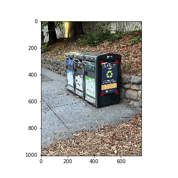
Berkeley Trashcan
Berkeley Trashcan (Keypoints)
Berkeley Trashcan (Rectified)
 Warp to: [(250, 200), (550, 200), (250, 700), (550, 700)]
Part 4: Mosaic Blending
Finally, we have everything we need to stich images together into a mosaic! To achieve this, we define correspondences to
represent exact matches within both images. After, we warp the first image to the second image's keypoints, then
align them together in a shared canvas. To eliminate harsh seams at the edges, we can use multi-resolution blending to
eliminate harsh seams at the edges of the image. This process is detailed below.
When each image is warped, we modify each image to have an alpha channel that indicates the pixels that are present
in the warped image. An alpha value of 0 indicates that no pixel is present (appears transparent) whereas an alpha value of 1
indicates that a pixel is present (actual image). As such, when blending two warped images together, we can utilize their alpha
channels to build a blending mask. This mask is generated by computing a distance transform
on the alpha channels of each warped image. The distance transform calculates
the closest distance of each non-zero pixel in the alpha channel to a pixel that has a value of 0. In other words, pixels that are close to the edge of the warped image will
have small distance transform values whereas pixels close to the center of the warped image will have large distance transform values. Any pixel outside of the
warped image has a distance transform value of 0 by default.
To perform multi-resolution blending, we split each image into their low and high frequency components.
Amazon Locker (Left)
Amazon Locker (Right)
Amazon Locker (Warped Left)
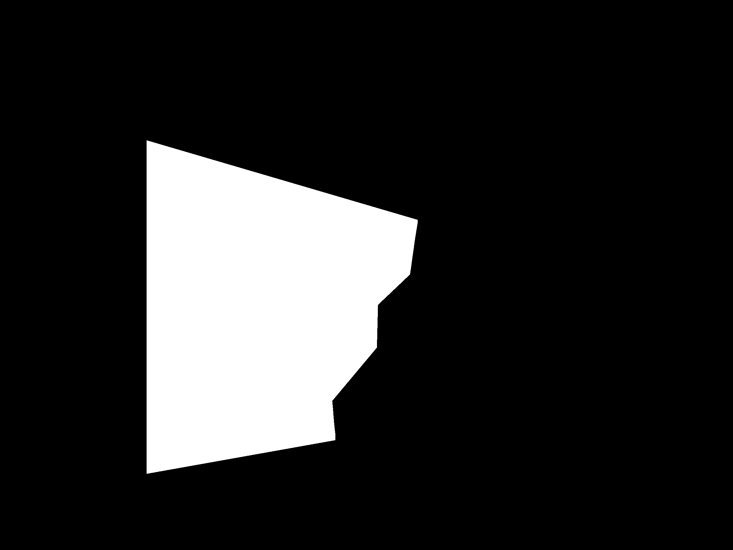
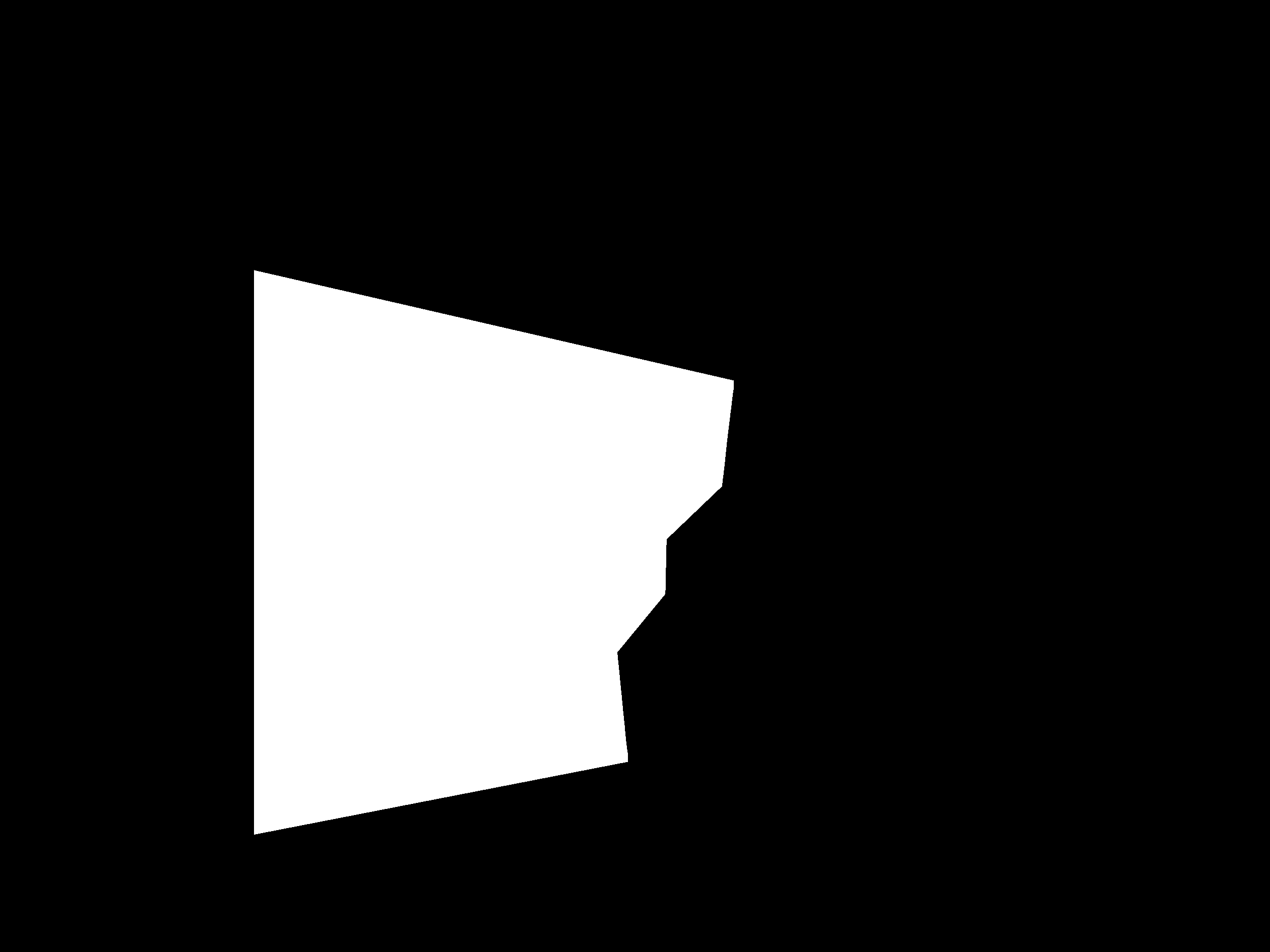
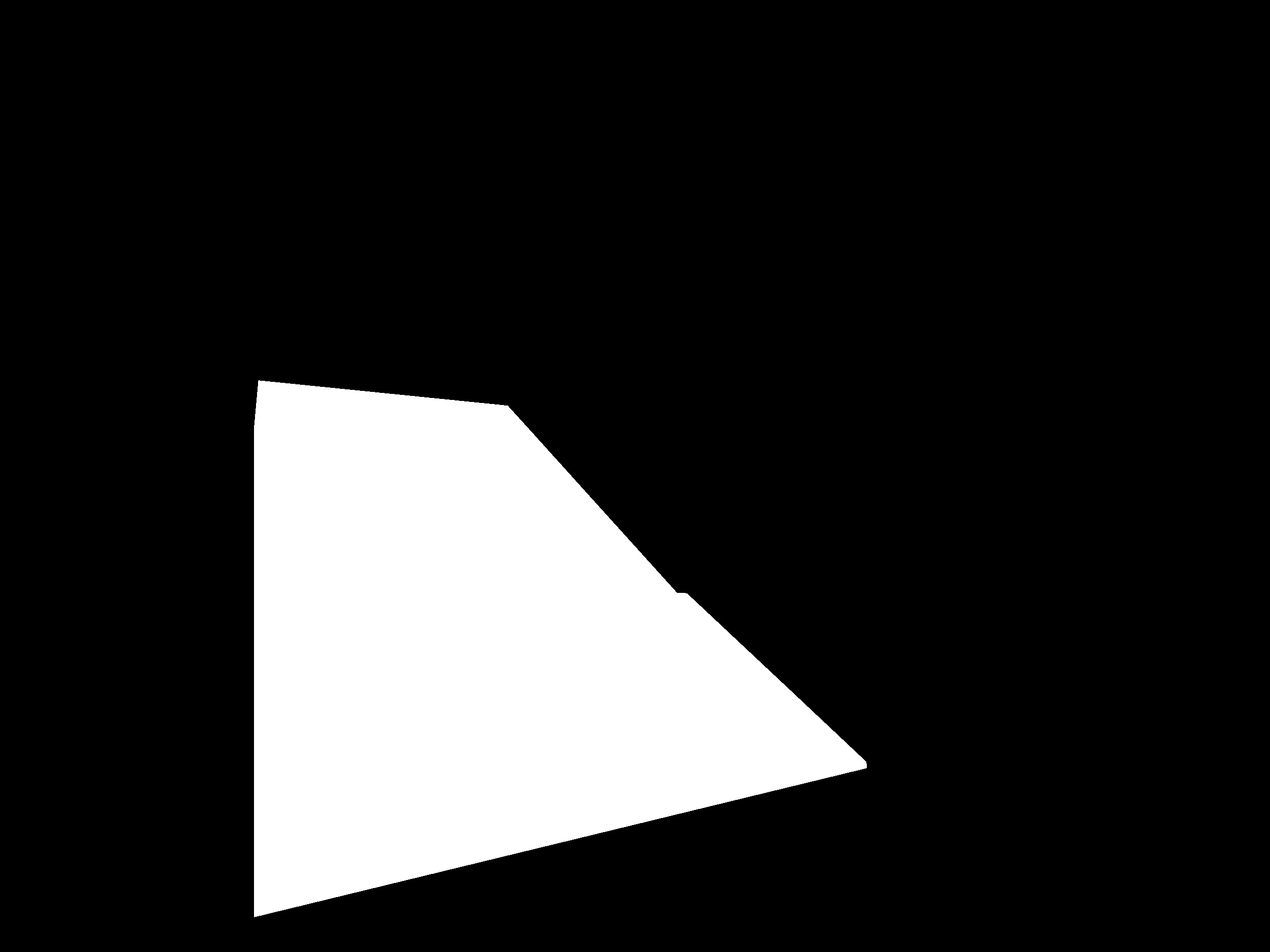
Blending Mask
Amazon Locker (Warped Right)
Amazon Locker Mosaic
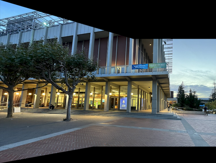
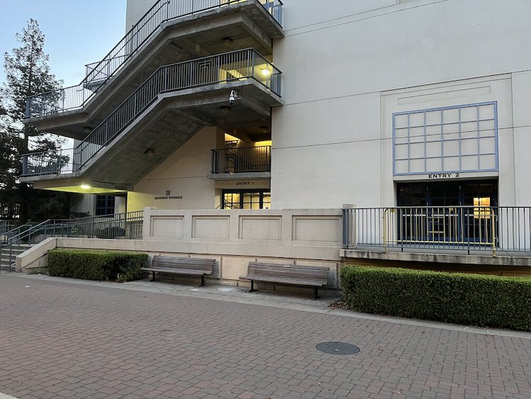
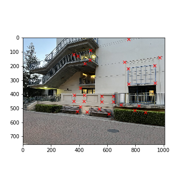
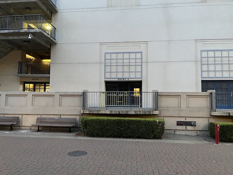
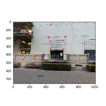
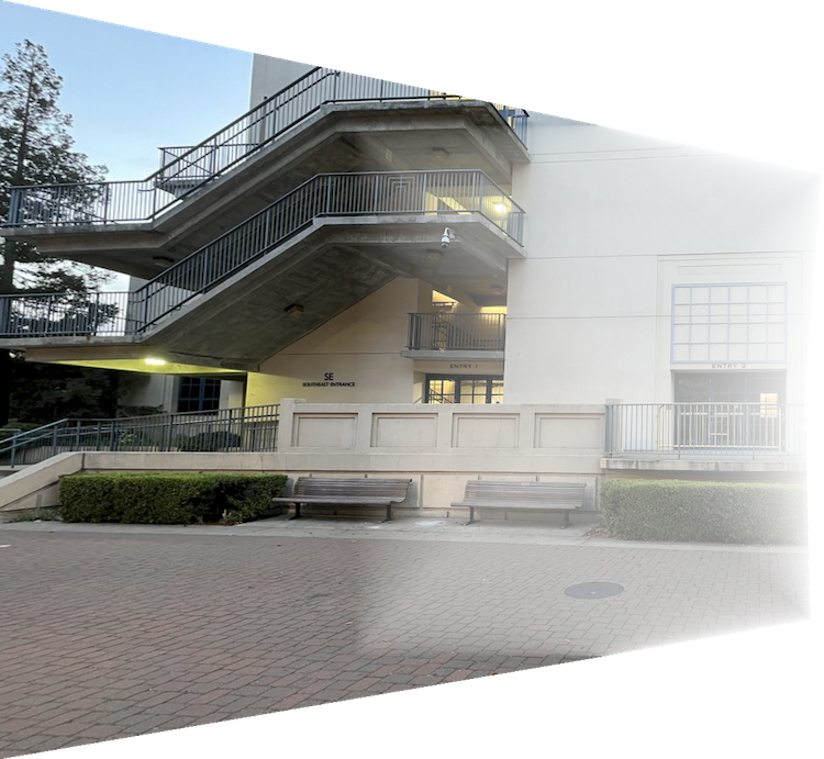
Haas Pavilion (Left)
Haas Pavilion (Right)
Haas Pavilion (Warped Left)
Blending Mask
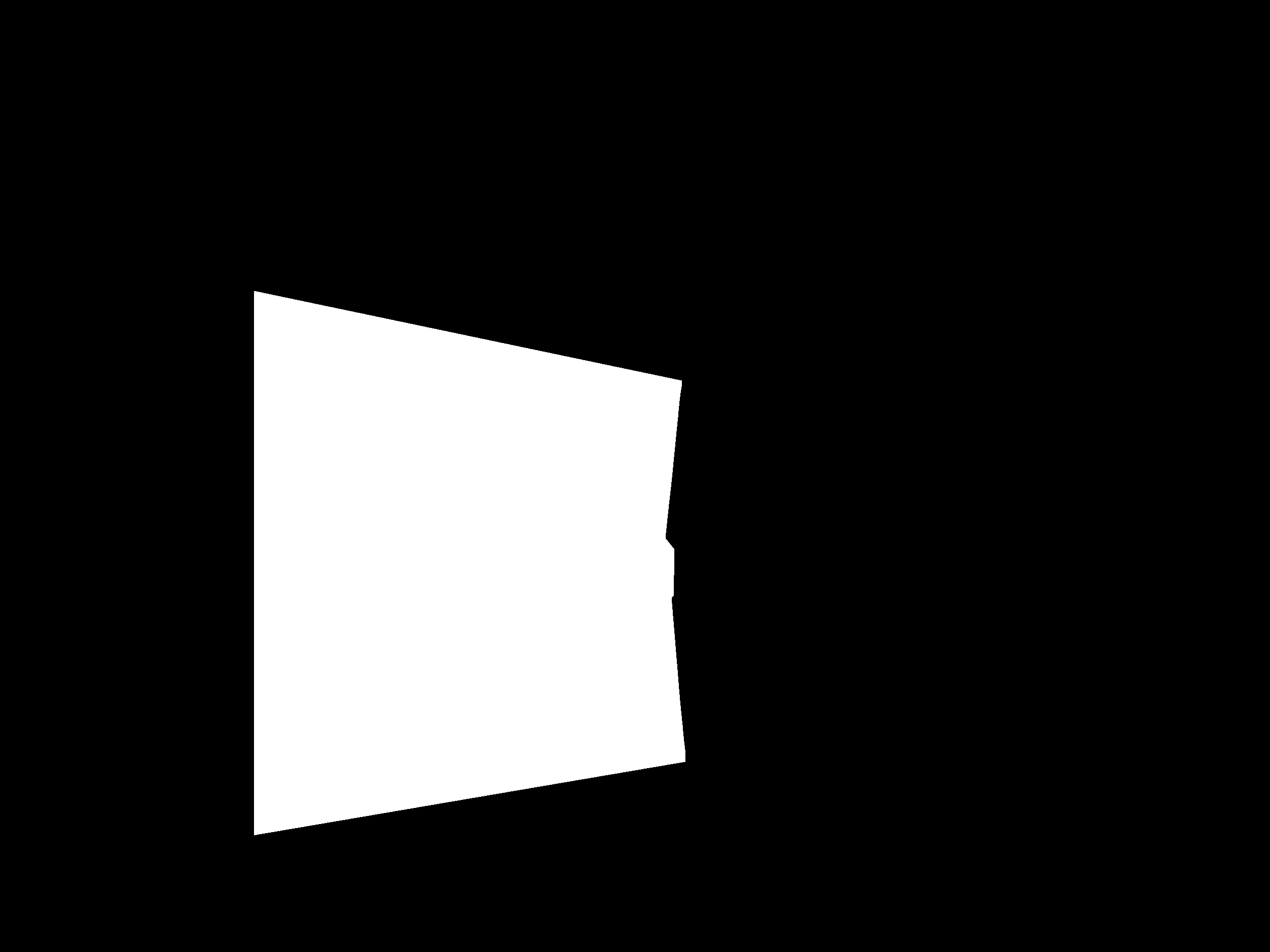
Haas Pavilion (Warped Right)
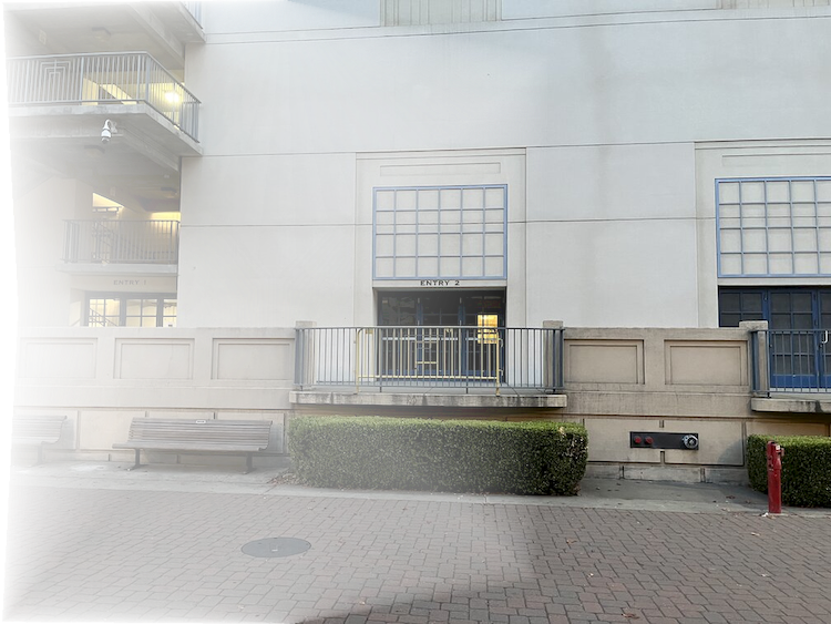
Haas Pavilion Mosaic
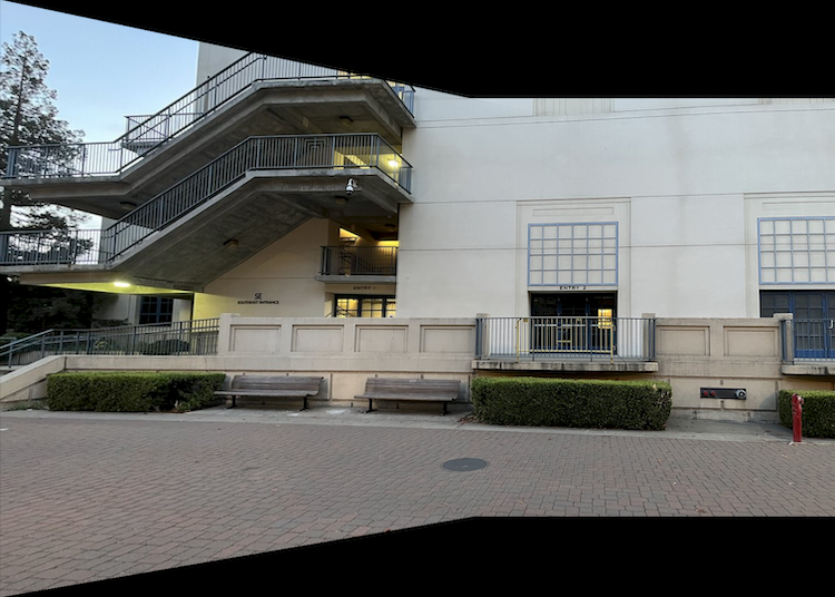
Bench (Left)
Bench (Right)
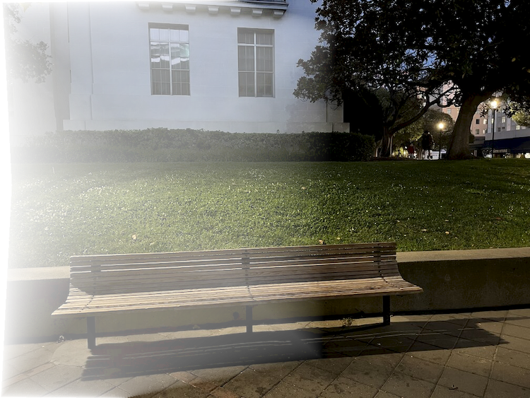
Bench (Warped Left)
Blending Mask
Bench (Warped Right)
Bench Mosaic
Tablet (Left)
Tablet (Right)
Tablet (Warped Left)
Blending Mask
Tablet (Warped Right)
Tablet Mosaic

In general, the final outputs look solid, with most of the overlapping components being blended together nicely and accounting for some lighting differences. There are a couple of slight artifacts along the edge of the intersection for a couple of the images, but overall they aren't very noticable and don't detract from the quality of the overall mosaics.
Phase A Takeaways
Overall, I thought this first phase was a nice introduction into the concept of homography and image stitching. In particular, I enjoy "rectifying"
different images to appear parallel to the front perspective, as it helped me understand how my PDF scanner app works: whenever I take a picture of
a document, it performs a perspective warp with homography to make the paper appear straight and readable.
One of my least favorite parts of this assignment, however, was having to manually select correspondences between both images, as any slight error in
the selection process would result in a misaligned mosaic. As such, I'm looking forward to the second part of this project where we'll be able to
automate this process!
Phase B: Feature Matching for Auto-Stitching
The main goal of this phase was to automate the selection of keypoints by implementing techniques outlined by this research paper. This process is outlined below.Part 1: Detecting Corner Features
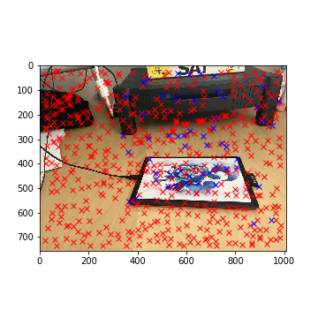
To detect the corner features of an image, we can use the Harris corner detector. In short, the Harris corner detector takes in a grayscale image and computes horizontal and vertical derivatives at each pixel along the image. It identifies a pixel as a "corner" if a pixel's derivative values are high. Note that I did not have to implement anything for this section: I utilized the Harris corner detector provided in the starter code.
Tablet Harris Corners (Left)
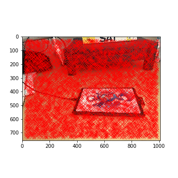
Tablet Harris Corners (Right)
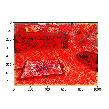
Although this is a good start, the Harris corner detector generates about 6000 detected corners for each image. As such, we need to filter out some of the corners.
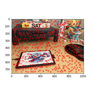
To do this, we can implement Adaptive Non-Maximal Suppression (ANMS). When generating Harris corners, each corner has an associated "strength" that indicates how strong
the corner is. Mathematically, given a function f that outputs the numerical "strength" of the corner, we assign each corner xi a radius ri where
ri = minj||xi - xj|| s.t. f(xi) < 0.9f(xj). After, we select the top 500 points that have the largest
radii values.
Intuitively, this attempts to identify corners that are one of the strongest within their respective cicle (significantly stronger points are outside of their "radius").
This allows us to filter points that are not only significant but also are distributed uniformly throughout both images. Note that 500 corners is still a lot of points,
but it's a step in the right direction! The results of running ANMS on both images is shown below.
Tablet Corners with ANMS (Left)
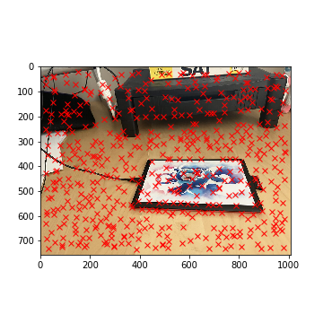
Tablet Corners with ANMS (Right)
Part 2: Extracting Feature Descriptors
Although we have generated 500 corners for both images, we still need to find a way to correspond keypoints between both images. This is where feature
descriptors come into play. To generate feature descriptors, we take a 40x40 segment around each corner (20 pixel radius) in the grayscale image, downsize
the descriptor to an 8x8 image, then bias-gain normalize it (in other words, given an 8x8 descriptor D, we calculate D' = (D - µ) / σ). These feature
detectors are known as MOPS, or "Multi-Scale Oriented Patches." An example of a MOP is shown to the right.
Through this process, each corner has a feature descriptor that uniquely identifies it.
Sample Point on Tablet
Descriptor

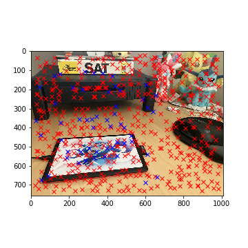
Part 3: Matching Feature Descriptors
In this part, we want to match feature descriptors from image 1 to feature descriptors to image 2. We can identify the closest feature detector by using some
type of similarity metric: for this project, I used SSD similar to what was described in Project 1.
As such, we would assign corners such that the SSD between both corners' corresponding feature descriptors was as small as possible.
However, this doesn't filter out bad matches, as this still leaves us with 500 paired corners. To resolve this issue, we implement Lowe's trick: for each feature descriptor Da
in image 1, find the 1st and 2nd closest feature descriptors Db1 and Db2 in image 2 that match image 1's feature descriptor.
Only keep this correspondance if ||Da - Db1|| / ||Da - Db2|| < T. In other words, we calculate the distance between the feature descriptor
from image 1 and its best matching feature descriptors in image 2 and ensure that Db1 matches Da significantly better than any other alternative feature
descriptors (i.e. second best and any other worse feature descriptor). For this step, I set T = 0.2.
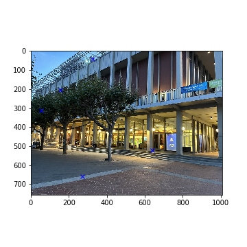
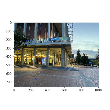
For the tablet example, the selected correspondances are highlighted in blue - this narrows down our matches to 54 corners.
Selected Tablet Corners with Lowe's (Left)
Selected Tablet Corners with Lowe's (Right)
Part 4: Computing the Homography with RANSAC
Although we could use our selected keypoints to compute the homography between both images, some of these matchings may not work (some feature descriptor matches can be misleading!). Our final simplification is to utilize RANSAC, or Random Sample Consensus, to choose the best point matchings to generate the warp. RANSAC implements the following algorithm:
- For n iterations:
- Select 4 random corresondances and compute the homography matrix H from them (as described earlier in the project).
- Generate a list of "inliers" that results from the homograph matrix H:
- For every point p1 in image 1:
- Calculate the warped position p2' of p1 by using the calculated homography matrix (p2' = H @ p1)
- Given the actual matching point p2 in image 2, if dist(p2 - p2') < e, add the point to the "inliers".
- During each iteration, keep the biggest list of inliers
- After n iterations, use the inliers as the correspondances for image warping.
Selected Tablet Corners with RANSAC (Left)
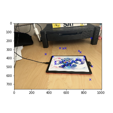
Selected Tablet Corners with RANSAC (Right)

Tablet Mosaic (Manual)
Tablet Mosaic (Auto)
Overall the results are very similar!
Part 5: Other Examples
Listed below are 2 other examples of using automated keypoints and how they compare to the original image (3 examples total). Note that the automatic alignments aren't perfect, but they are still pretty close to their manually-aligned counterparts.
Haas Pavilion Mosaic (Manual)
Haas Pavilion Mosaic (Auto)
Bench Mosaic (Manual)
Bench Mosaic (Auto)

Note that the Amazon Lockers example was omitted from automatic stitching. Since both images were very complex with many details (doors, trees, second-floor fences, lighting differences, etc), the automatic algorithm failed to match feature descriptors correctly between both images. The final 5 points generated by RANSAC show no similarities whatsoever. Some images are displayed below to showcase these errors.
Selected Amazon Corners with RANSAC (Left)
Selected Amazon Corners with RANSAC (Right)
Sample Amazon Point (Left)

Descriptor (Left)

Sample Amazon Point (Right)
Descriptor (Right)

Auto Amazon Merged
Phase B Takeaways
Overall, I thought it was intriguing how we could combine a series of simple steps to achieve something as complex as selecting correspondances between two simliar images. I found implementing ANMS to be the most satisfying, as the algorithm itself was very intuitive and resulted in the largest keypoint simplification (from thousands of keypoints to only hundreds). However, I also learned that this algorithm has some limitations: its inability to merge complex images like the Amazon Lockers example resulted from being unable to match similar features by using MOPS. Nevertheless, this algorithm is very good for something that was conceptualized in the early 2000s, as some of the auto-stitched examples are much more effective than my manual attempts.
(Note: some of the images were resized to fit the 25MB file limit)