Motivating Example: CAT Scan Imaging

Linear Equations > Motivating example | Existence, Unicity | Solving via QR | Applications

Overview
From 1D to 2D: axial tomography
Linear equations for a single slice
Issues raised: finding a solution, existence and unicity

Overview

Tomography means reconstruction of an image from its sections. The word comes from the greek ‘‘tomos’’ (‘‘slice’’) and ‘‘graph’’ (‘‘description’’). The problem arises in many fields, ranging from astronomy to medical imaging.

Computerized Axial Tomography (CAT) is a medical imaging method that processes large amounts of two-dimensional X-ray images in order to produce a three-dimensional image. The goal is to picture for example the tissue density of the different parts of the brain, in order to detect anomalies (such as brain tumors).

Typically, the X-ray images represent ‘‘slices’’ of the part of the body (such as the brain) that is examined. Those slices are indirectly obtained via axial measurements of X ray attenuation, as explained below. Thus, in CAT for medical imaging, we use axial (line) measurements to get two-dimensional images (slices), and from that scan of images, we may proceed to digitally reconstruct a three-dimensional view. Here, we focus on the process that produces a single two-dimensional image from axial measurements.

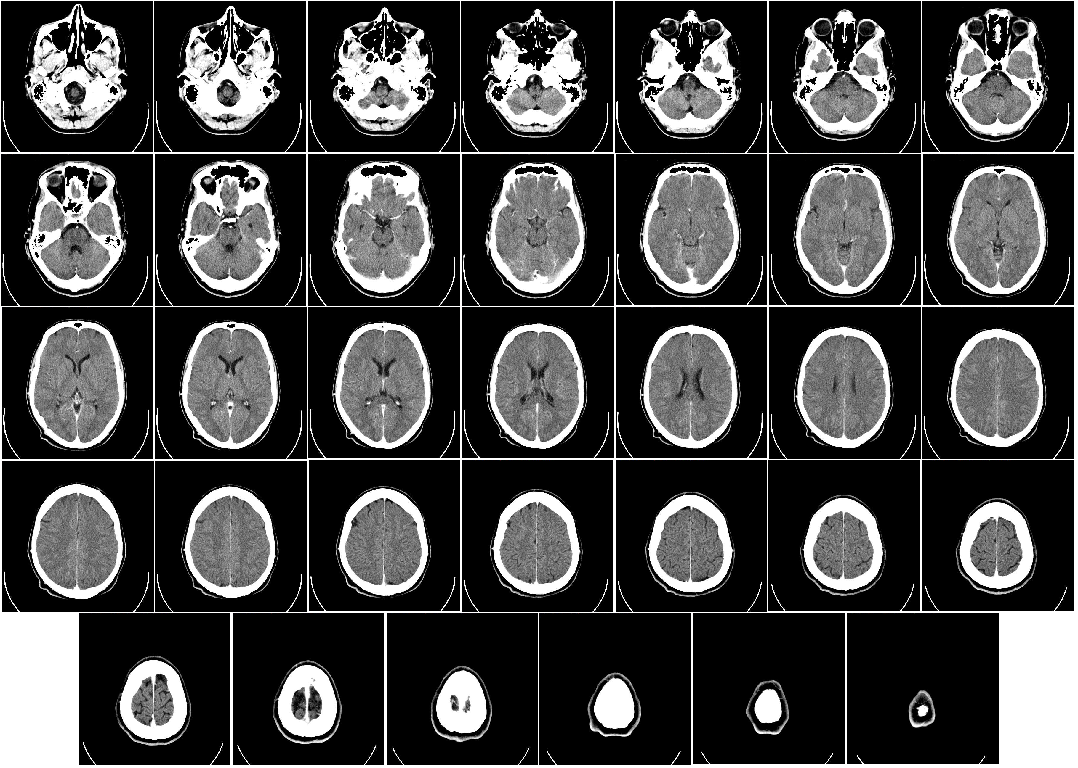A collection of ‘‘slices’’ of a human brain obtained by CAT scan. The pictures offer an image of the density of tissue in the various parts of the brain.

Each slice is actually reconstructed image obtained by a tomography technique explained below. The collection of slices can in turn be used to form a full three-dimensional representation of the brain.

Source: Wikipedia entry.

From 1D to 2D: axial tomography

In CAT-based medical imaging, a number of X rays are sent through the tissues to be examined along different directions, and their intensity after they have traversed the tissues is captured by a camera. For each direction, we record the attenuation of the X ray, by comparing the intensity of the X ray at the source, $I_{rm source}$ , to the intensity after the X ray has traversed the tissues, at the receiver's end, $I_{rm rec}$ .

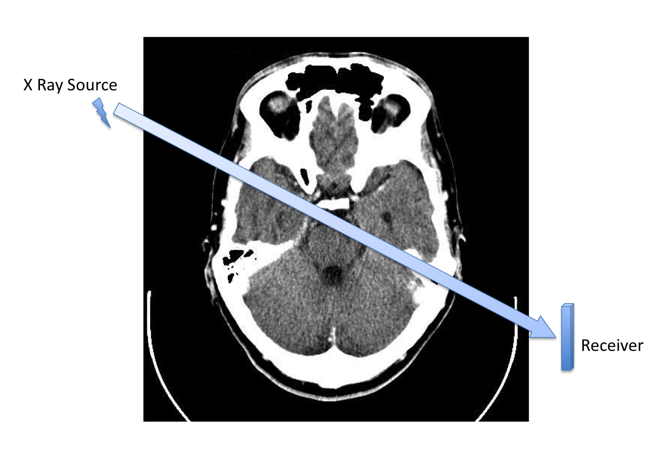A single slice obtained by CAT scan. Each slice is a reconstructed image obtained by recording the attenuation of x-rays through the tissues along a vast number of directions. The picture shows the X Ray source and the corresponding receiver used to measure attenuation along a specific direction.

Linear equations for a single slice

Similar to the Beer-Lambert law of optics, it turns out that, to a reasonable degree of approximation, the log-ratio of the intensities at the source and at the receiver is linear in the densities of the tissues traversed.

We consider a discretized version of a square slice image, with N times N pixels of gray scale values. On the example pictured here, we simply have N=2 , and a total of four pixels. Each pixel can be represented by an index pair (i,j) , with 1 le i,j le N . The gray scale values represent the density of the tissues, with $d_{ij}$ the density at pixel (i,j) .

With the discretization, the linear relationship between intensities log-ratios and densities can be expressed as

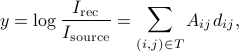
$y = log frac{I_{rm rec}}{I_{rm source}} = sum_{(i,j) in T} A_{ij} d_{ij} ,$

where denotes the indices of pixel areas traversed by the X ray, $d_{ij}$ the density in the (i,j) area, and $A_{ij}$ the proportion of the area within the pixel that is traversed by the ray.

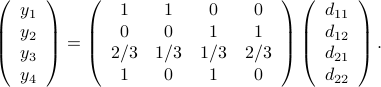
Linear relationship between the observed log-intensity ratios y_1,y_2,y_3,y_4 and (unobserved) densities $d_{ij}$ , 1 le i,j le 2 within the four pixels. The slanted arrow corresponds to an X ray which traverses about 2/3 of the area of pixels (1,1) and (2,2) , and 1/3 of the areas of the pixels (1,2) and (2,1) .

Thus, we can relate the vector $d in mathbf{R}^{N^2}$ to the observed intensity log-ratio vector $y in mathbf{R}^m$ in terms of a linear equation

where $A in mathbf{R}^{n times m}$ , with n := N^2 . Note that depending on the number of pixels used, and the number of measurements, the matrix can be quite large. In general, the matrix is wide, in the sense that it has (many) more columns than rows ( n >> m ). Thus, the above system of equations is usually undetermined.

In the example pictured above, we have

$left(begin{array}{c} y_1 y_2 y_3 y_4 end{array}right)= left(begin{array}{cccc} 1 & 1 & 0 & 0 0 & 0 & 1 & 1 2/3 & 1/3 & 1/3 & 2/3 1 & 0 & 1 & 0 end{array}right) left(begin{array}{c} d_{11} d_{12} d_{21} d_{22} end{array}right) .$

Issues

The above example motivates us to address the problems of solving linear equations. It also raises the issue of existence (do we have enough measurements to find the densities?) and unicity (if a solution exists, is it unique?).