Existence, Unicity
Set of solutions to a linear equations
Existence: the range and rank of a matrix
Unicity: the nullspace and nullity of a matrix
Fundamental facts about range and nullspace
Consider the linear equation in  :
:

where  and
and  are given, and is the variable.
The set of solutions to the above equation, if it is not empty, is an affine subspace. That is, it is of the form  where
where  is a subspace.
We'd like to be able to
determine if a solution exists;
if so, determine if it is unique;
compute a solution
 if one exists;
find an orthonormal basis of the subspace
.
Existence: range and rank of a matrix
Range
The range (or, image) of a  matrix
  is defined as the following subset of
  :
:

The range describes the vectors  that can be attained in the output space by an arbitrary choice of a vector
  in the input space. The range is simply the span of the columns of .
If  , we say that the linear equation
  is infeasible. The set of solutions to the linear equation is empty.
The matlab function orth accepts a matrix as input, and returns a matrix, the columns of which span the range of the matrix , and are mutually orthogonal. Hence,  , where
  is the dimension of the range. One algorithm to obtain the matrix
  is the Gram-Schmidt procedure.
>> U = orth(A); % columns of U span the range of A, and U'*U = identity
Example:
Rank
The dimension of the range is called the rank of the matrix. As we will see later, the rank cannot exceed any one of the dimensions of the matrix :  . A matrix is said to be full rank if
  .
.
r = rank(A); % r is the rank of A
Note that the rank is a very ‘‘brittle’’ notion, in that small changes in the entries of the matrix can dramatically change its rank. Random matrices, such as ones generated using the Matlab command rand, are full rank. We will develop here a better, more numerically reliable notion.
Examples:
Range and rank of a simple matrix.
Full row rank matrices
The matrix is said to be full row rank (or, onto) if the range is the whole output space, . The name ‘‘full row rank’’ comes from the fact that the rank equals the row dimension of . Since the rank is always less than the smallest of the number of columns and rows, a matrix of full row rank has necessarily less rows than columns (that is,  ).
).
An equivalent condition for to be full row rank is that the square,  matrix
  is invertible, meaning that it has full rank,
  . Proof.
Unicity: nullspace of a matrix
Nullspace
The nullspace (or, kernel) of a matrix is the following subspace of  :
:

The nullspace describes the ambiguity in given : any  will be such that
  , so cannot be determined by the sole knowledge of
  if the nullspace is not reduced to the singleton
  .
.
The matlab function null accepts a matrix as input, and returns a matrix, the columns of which span the nullspace of the matrix , and are mutually orthogonal. Hence,  , where
  is the dimension of the nullspace.
U = null(A); % columns of U span the nullspace of A, and U'*U = I
Example:
Nullspace of a simple matrix.
Nullity
The nullity of a matrix is the dimension of the nullspace. The rank-nullity theorem states that the nullity of a matrix is  , where is the rank of .
Full column rank matrices
The matrix is said to be full column rank (or, one-to-one) if its nullspace is the singleton . In this case, if we denote by  the
the  columns of , the equation
has  as the unique solution. Hence, is one-to-one if and only if its columns are independent. Since the rank is always less than the smallest of the number of columns and rows, a matrix of full column rank has necessarily less columns than rows (that is,
  ).
).
The term ‘‘one-to-one’’ comes from the fact that for such matrices, the condition  uniquely determines , since
  and
and  implies
 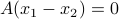 , so that the solution is unique:
  . The name ‘‘full column rank’’ comes from the fact that the rank equals the column dimension of .
An equivalent condition for to be full column rank is that the square,  matrix
  is invertible, meaning that it has full rank, . (Proof)
Example: Nullspace of a transpose incidence matrix.
Fundamental facts
Two important results about the nullspace and range of a matrix.
The nullity (dimension of the nullspace) and the rank (dimension of the range) of a matrix add up to the column dimension of , .
Another important result is involves the definition of the orthogonal complement of a subspace.
The range of a matrix is the orthogonal complement of the nullspace of its transpose. That is, for a matrix :
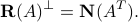
|
|
The figure provides a sketch of the proof: consider a 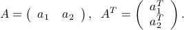
Then |
 matrix, and denote by
  (
( ) its rows, so that
 if and only if
  ,
,  if and only if it is orthogonal to the vectors