Outer Spherical Approximations
Outer spherical approximation via gridding
Outer spherical approximation via Lagrange relaxation
Improved spherical approximation via affine Lagrange multipliers
Let us consider a candidate sphere  , of center
  and radius
  . We formulate the condition that the sphere contains the intersection of all the spheres of center
  , as follows:

This conditions appears to be hard to check.
Outer spherical approximation via gridding
A first approach, which works well only in moderate dimensions (2D or 3D), simply entails gridding the boundary of the intersection. In 2D, we can parametrize the boundary explicitly, as a curve, using an angular parameter. For each angular direction ![theta in [0,2pi]](eqs/1626472798141214711-130.png) , we can easily find the point that is located on the boundary of the intersection, in the direction given by
, we can easily find the point that is located on the boundary of the intersection, in the direction given by  : we simply maximize
  such that the point
  is inside everyone of the spheres. (There is an explicit formula for the maximal value.)
One we have computed  points on the boundary,
  ,
,  , we simply solve the SOCP

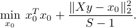
The gridding approach suffers from the fact that we need to grid finely to be able to guarantee that the spherical approximation we are computed indeed contains all the points on the intersection. On the other hand, too fine a grid results in a large number of constraints, which in turn adversely impacts the time needed to solve the above problem.
 |
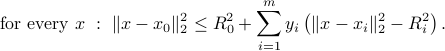
Outer spherical approximation to the intersection via gridding. This provides an estimated point (the center of the outer shpere), with an estimate of the uncertainty around it. We have used only |
 points on the boundary to enforce the constraint that the outer sphere contains the intersection. As a result, our approximation is not really an outer approximation, as it does not contain all the intersection points.
 |
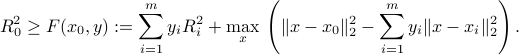
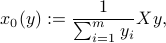
Outer spherical approximation to the intersection via gridding. Here we have used 63 points on the boundary. The approximation can now be termed an outer approximation as it (almost!) does not leave out any point in the intersection. |
Outer spherical approximation via Lagrange duality
We now develop an alternate approach which relies on weak duality concepts.
A sufficient condition
A sufficient condition for the above condition  to hold is that there exist a non-negative vector
  such that
Indeed, it is easily checked that if a point  belongs to all the spheres, then indeed the sum above is less or equal than
  when
when  .
.
Minimizing the radius  subject to the condition that the above holds for some will result in a conservative (larger) estimate of the amount of uncertainty.
SOCP formulation
Alternatively we can express the above condition as:
The problem of minimizing the radius subject to the above condition can thus be written as
It turns out that we can express the function  in closed-form, as proven here:
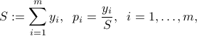
where for notational convenience we use the matrix  and the vector
  with components
  ,
,  . (Remember that our measurement consistency condition holds, so that
  .)
.)
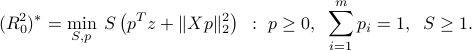
We are led to consider the sub-problem of minimizing over , with  fixed. If
  , then we must have
  . If
. If  , must solve
Again, this a convex quadratic problem, with a (unique) solution obtained by taking derivatives. A minimizer is  , where
that is, is the weighted average, with weights given by  , of the points
  . Note that the expression remains valid when
  , since then we must have .
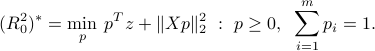
Plugging the above value of in the problem leads to a problem in variable only:
The above problem can be solved as an SOCP with rotated second-order cone constraints:
A simpler formulation (consistent measurements)
We can obtain a simpler formulation that involves QP only. We now use our measurement consistency assumption, which translates as . First we replace the variable with two new variables  , and a new constraint. The new variables are defined as
and the new constraint is  . We obtain the new problem
Since , the term inside the parentheses is non-negative, and thus  is optimal. Hence the problem reduces to a QP:
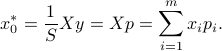
This provides the optimal radius. The optimal point is
 |
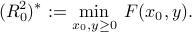
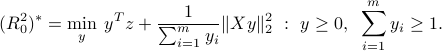
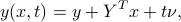
Outer spherical approximation via Lagrange duality. This provides an estimated point (the center of the outer sphere), with an estimate of the uncertainty around it. The approximation is very conservative. |
An improved condition via affine duality
To improve our condition, we start from the equivalent condition for intersection containment:

We now consider a relaxed of the form

where  , and the
  's are now non-negative functions of
  . (Before, we chose them to have constant values.) The above is still hard to check in general, but becomes easy if we make the assumption that the functions
 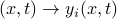 are affine.
We proceed by taking the vector 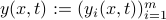 to be of the form
where  ,
,  and
and  will be variables. (The case before will be recovered upon setting
  ,
,  .)
.)
The condition above becomes a single quadratic condition on :

The above can be equivalently expressed as a positive semi-definiteness condition on a symmetric matrix that is affine in  :
:

It remains to express the condition that the affine functions  should be non-negative on the intersection. Precisely, we seek to enforce that for every
 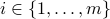 , the condition

holds (here,  stands for the
  -th column of matrix
  ). Now, we apply direct Lagrange duality. A sufficient condition for the above to hold is that there exist non-negative numbers
  ,
,  , such that

Again, the above is equivalent to a single linear matrix inequality in the variables and :
Putting this together, we obtain the SDP in variables  :
:
![min : R_0^2 ~:~ begin{array}[t]{l} left( begin{array}{ccc} nu^Tmathbf{1} & -nu^TX^T+frac{1}{2}mathbf{1}^TY^T & frac{1}{2}(mathbf{1}^Ty - nu^Tz -tau-1) -Xnu-frac{1}{2}Ymathbf{1} &tau I - YX^T-XY^T & x_0 - Xy - frac{1}{2}Yzfrac{1}{2}(mathbf{1}^Ty - nu^Tz -tau-1) & (x_0 - Xy - frac{1}{2}Yz)^T & R_0^2 - y^Tz-eta end{array}right) succeq 0, ;; eta ge x_0^Tx_0 left( begin{array}{cc} nu_i - sum_{j=1}^m N_{ij} & frac{1}{2} Y_i - sum_{j=1}^m N_{ij}x_j (frac{1}{2} Y_i - sum_{j=1}^m N_{ij}x_j)^T & y_i - sum_{j=1}^m N_{ij} z_j end{array}right) succeq 0, ;; i=1,ldots,m, end{array}](eqs/3393953924836324334-130.png)
 |
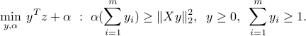
Improved outer spherical approximation via affine Lagrange duality. The refined approximation is now exact, in contrast with the previous approximation. The improvement is due to the fact that our relaxation involves Lagrange dual variables that are not constant anymore, but are affine in the primal variables. |