Consistency

The measurements may not be consistent, in the sense that the intersection of all the spheres may be empty. Here, we first address the problem of checking consistency, and adjust our measurements if necessary.

Checking consistency

We begin by checking if our consistency condition holds. This can be formulated as an optimization problem, involving no (or, zero) objective:

The above is an SOCP. On exit, a solver such as CVX will provide either a feasible point , or determine (unambiguously) that there is no feasible point.

% input: 2xm data matrix X, m-vector of radiuses R
% output: feasible point xfeas, empty if intersection is empty
cvx_begin
    variable xfeas(2,1)
    minimize( 0 )
    subject to
        for i = 1:m,
		R(i) >= norm(xfeas-X(:,i),2);
	end
cvx_end
if ~isfinite(cvx_optval), xfeas = []; end

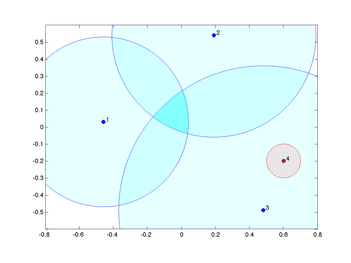Localization problem with one range measurement added, with data 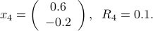This last measurement (in red) corresponds to a faulty sensor, and makes the measurements inconsistent. Solving the above problem with CVX return an infeasibility message, and the optimal value is .

Adjusting inconsistent measurements

If there is no feasible point, we may want to modify our range measurements so that they become consistent. A variety of approaches are possible. Clearly, increasing the distances will, at some point, make the problem feasible. Let us find the smallest increases that result in a non-empty intersection. We are led to the problem

The above problem can be expressed as an SOCP, when the norm chosen is one of the three popular norms (, , or Euclidean). The qualitative behavior of the solution depends on the choice of the norm.

If the norm chosen is the Euclidean one, we are minimizing the sum of the squares of the adjustments (increases) that are necessary to make our measurements consistent. This results in non-zero adjustments for all the measurements, and the new (unique) intersection point (in green) is far away from the initial intersection.

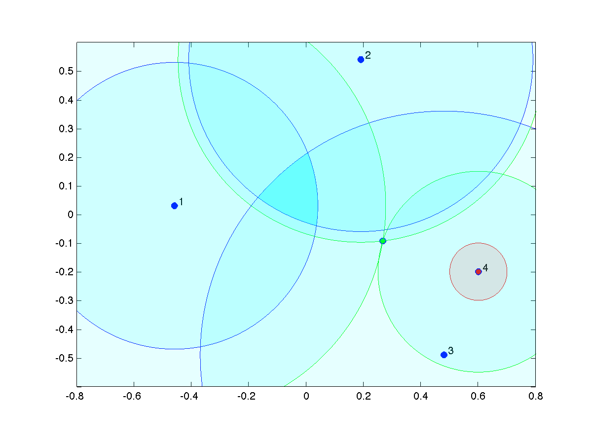
Choosing an norm will tend to make the smallest number of adjustment necessary. This would make sense if we believe that a few of our measurements are outliers, and due to faulty sensors.

Identifying a faulty sensor that resulted in inconsistent measurements: here we have solved the minimum -norm of adjustments necessary to make the measurements consistent. The approach identifies the offending measurement, since the optimal adjustment vector is almost zero except for its last component, which corresponds to the fourth sensor. We observe, however, that the indentification is not perfect, as the measurement of sensor 1 is also adjusted, albeit only slightly. This is due to the fact that the -norm approach is a only a heuristic to solve cardinality minimization problems, as seen here.

In the above problem, the sign constraint on implies that we assume that a fault in a sensor only results in under-estimating the radius (hence to a possible infeasible problem). We can remove the sign constraint if we want to address a problem of faulty sensors, where some of them over-estimate the radius measurement.

The above approach will in general make the smallest adjustments necessary. This means that in general at the outset of solving the problem, the intersection reduces to a single point (the optimal variable delivered by the above procedure). We can choose that point to be our estimate. However, if indeed we suspect some faulty sensors, it may not make sense to proceed that way. Instead, we may use the above problem (with -norm objective) as a method to detect faulty sensors (those for which at optimum). Then, we remove those faulty sensors from the problem, and proceed with a set of consistent measurements.

Assumption: consistent measurements

From now on, we assume that our measurements are consistent. Without loss of generality, we may translate the whole problem so that the feasible point that proves consistency, , is zero. This means that the vector with components , , is non-negative componentwise ().